
Word Embeddings in Large Language Models: Part 1
Methods to construct word embeddings


TL;DR
Word embeddings lie at the heart of Generative AI (GenAI) and many of its most popular applications, such as those based on Retrieval Augmented Generation (RAG). This is the first post in a two-part series, where I first define embeddings, and then present the different ways we can represent words (sparse vs. dense, and static vs. dynamic). As usual, you can follow all of the calculations with the code be found in this Google Colab notebook.
Defining word embeddings
Embeddings are numerical representations of each word, and capture the meaning of the word in their context.1 This concept is based on the distributional hypothesis, which posits that words appearing in the same context are likely to be “similar”. Alternatively, the distributional hypothesis suggets that we can infer the meaning of a word by looking at its neighboring words.
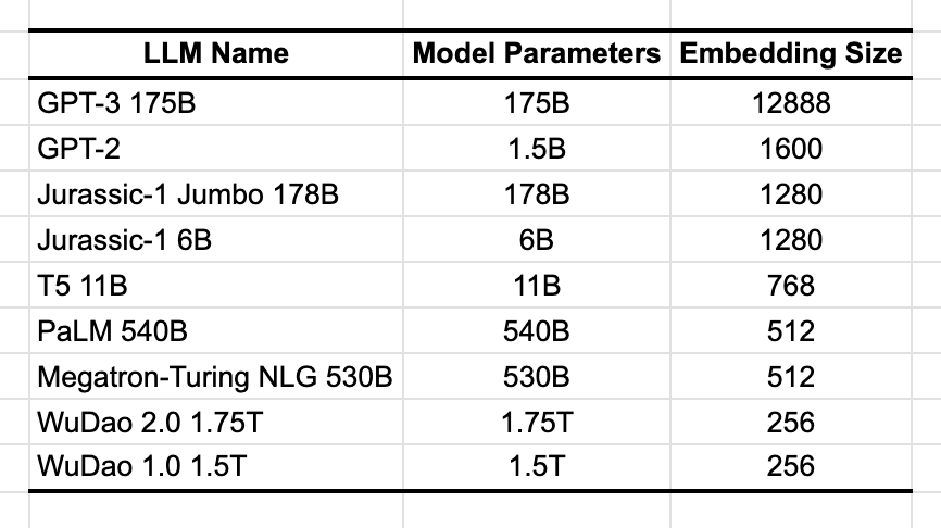
Since large language models (LLMs) use words as inputs, these must first be converted to numbers before passing through the model’s architecture. Most commonly, words are mapped into vectors of size d, and this is a metaparameter that varies across models (Table 1). For instance, the largest version of GPT-3 converted words to vectors with 12.8K elements. But for most smaller models this parameters is in the hundreds.
In Figure 1 I show how this actually looks like. You start by creating the vocabulary for the model, listing all unique entries in the corpus. These words are then mapped into vectors. In the figure I use 8-dimensional vectors, but as was just seen, the dimension is usually in the hundreds or thousands. Intuitively speaking, the larger the dimension the richer the representation.

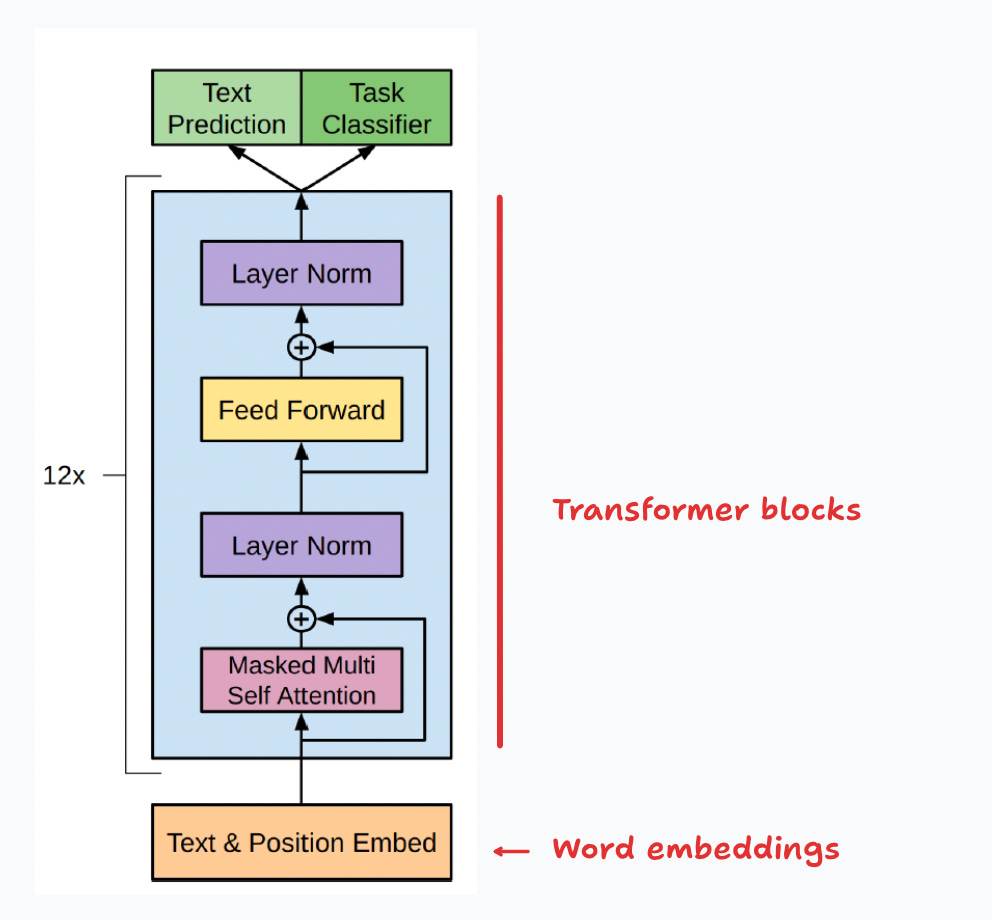
Since embeddings transform input words, they typically lie at the “bottom” of a deep neural network. For instance, in models like the GPTs, these vectors are used as inputs to the first of the transformer blocks (Figure 2). Just as all of the other parameters, the embeddings are learned by the algorithm.
In many applications embeddings have no intrinsic use. Rather, at inference time, these, and all other model parameters, are used to make a prediction. But there are many other applications where embeddings are of intrinsic use. These applications will be discussed in the second part of this series.
Retrieval Augmented Generation (RAG)
I’ve proposed before that one of the underlying capabilities of GenAI is the property of information retrieval (Figure 3). Thanks to the extensive dataset used to train these LLMs, many times the model provides accurate answers to questions across many different domains. However, it’s not uncommon that models hallucinate and generate inaccurate responses when the question wasn’t clear enough, or when it just doesn’t have a way to know the answer. Prompt engineering is important to deal with the former, and RAG is a useful alternative in the latter cases.

A typical use case for RAG is when building a chatbot for your customers. Since most of the relevant information is internal to the company, ChatGPT has no way to provide accurate answers to many of your customers’ queries. In situations like these, RAG, and word embeddings, come to the rescue.
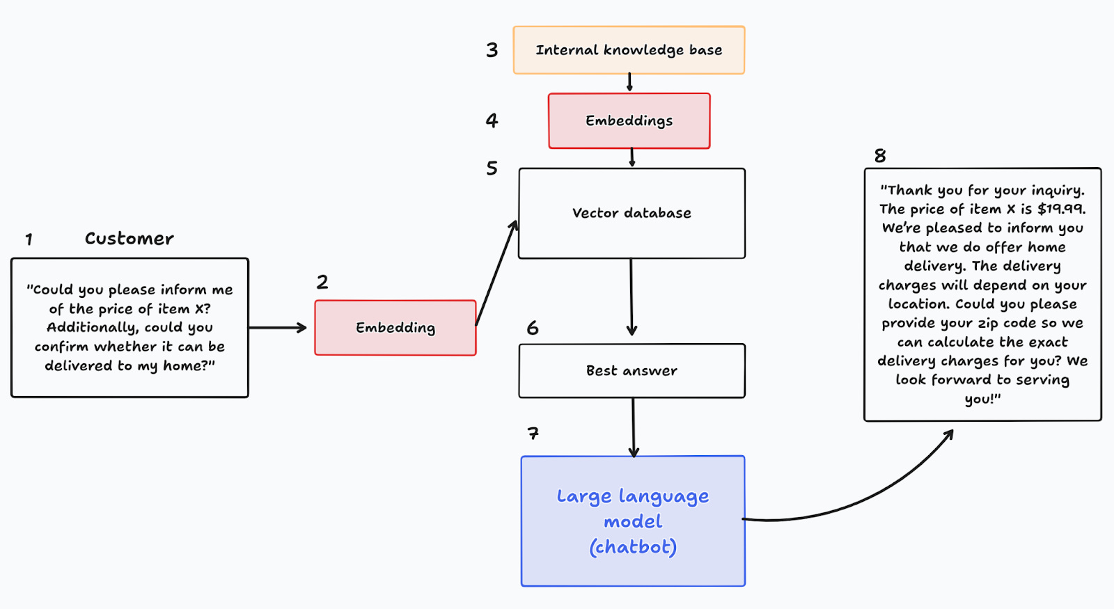
Figure 4 shows how this is typically implemented. A customer asks a question (1), which is then transformed to an embedding (2). Prior to the implementation, the company had organized an internal knowledge base and transformed all of its entries into embeddings (3-4). These are then stored in a vector database (5). Vector databases are optimized to find the most similar entry in the knowledge base given a query, and thus, it provides the best answer to the question, given the knowledge base and the embeddings (6). This answer is then passed in an augmented prompt to the LLM (7), which finally generates an answer to the customer (8).
Note that embeddings play a critical role in this design: they transform the query and the knowledge base, and are used to find the best answer. This highlights one of the key features of embeddings: they capture the semantic content of words, and map it into a space where standard arithmetic operations are performed. For instance, we can very quickly find measures of similarity, as we will explore shortly.
Types of word embeddings
Broadly speaking, there are two types of word embeddings: sparse or dense embeddings, and the latter category can be split into static and dynamic or contextual embeddings. I will now describe each of these.

Sparse embeddings
The first two methods used to construct sparse are the term-document and term-term matrices. It’s common to start with a set of documents, each containing different words. To compute the term-document matrix, you count the number of occurrences of each word in each document, and the result is then mapped to the corresponding element in a matrix.
In Figure 6 I show a term-document matrix for the 17 blog posts I’ve written. For instance, I used the term “data” 23 times in the post on the importance of managers in data teams, 12 times in the post on feature importance, and so on. There’s one row for each unique word that appear in the vocabulary. It’s a good practice to do some preprocessing of the data, such as dropping stop words and some non-alphanumeric tokens, or stemming and lemmatization. With the latter, words like “figure” and “figures” are taken as one word.

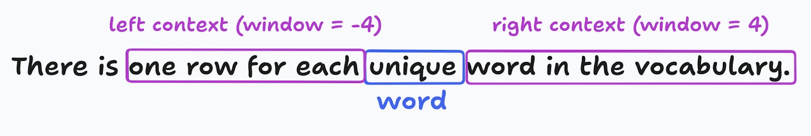
The term-term matrix is handy to move closer to local context, instead of the broader space of “documents”. As the name suggests, this is a square matrix of dimension VxV (V is the size of the vocabulary), where we count co-occurrences of words within a context, defined by a surrounding window. In Figure 7 I show this with the sentence “There is one row for each unique word in the vocabulary”.
In Figure 8 I show the first 5 rows and a few of the columns of the 2245 x 2245 term-term matrix computed using the blog posts and a window of 6 words. To see why these are called sparse embeddings, note that the matrix has a large percentage of zeros (97.5%). This is quite common with term-document and term-term matrices.

One problem with the term-document matrix is that common words, which appear in many documents, may not be as informative about the semantic content of a given document. For instance, consider the words “data” and “vector”. Since I write about data science, the former appears in most of my posts, and thus provides little information about the actual contents of a specific post. On the other hand, less frequent words like “vector” have a larger information content. The term frequency -inverse document frequency matrix (TF-IDF) takes care of these cases.
The TF part corresponds to the counts already encountered in the term-document matrix (with a log transformation). On the other hand, the document-frequency (DF) quantifies the fraction of documents that include a word across all documents. The IDF gives a higher weight to words that appear in fewer documents, and may thus be more informative.
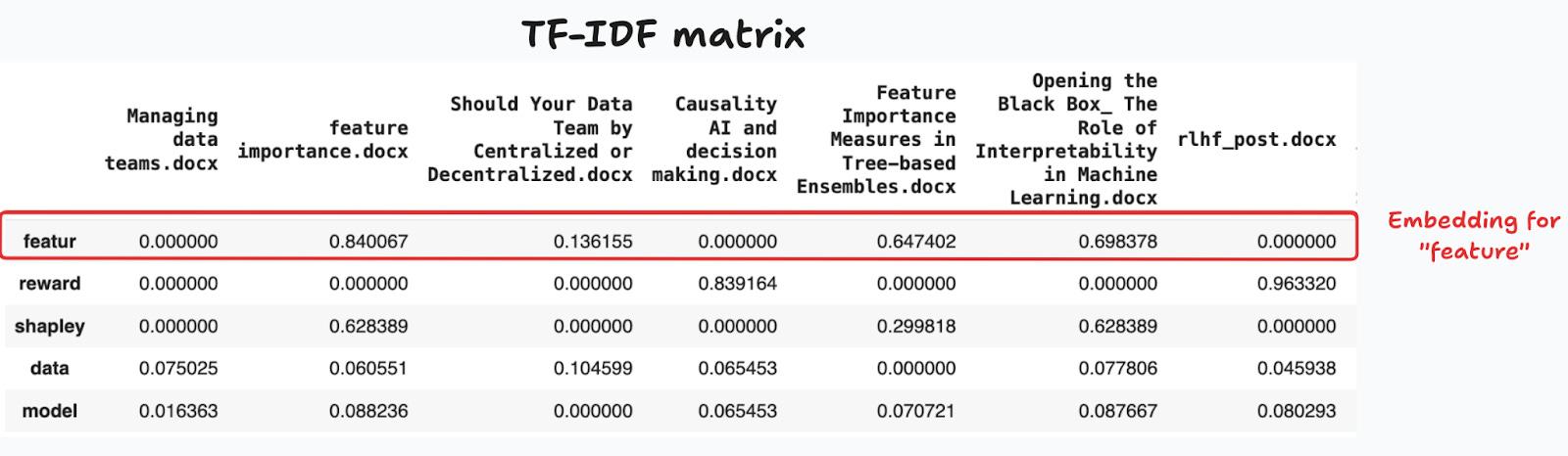
Figure 9 shows the first rows for some of the words that have large and low tf-idf values across all blog posts. Words like “feature”, “reward” and “shapley” are highly informative, while “data” and “model” appear in most blog posts, and thus carry less information content and lower tf-idf values.
The Pointwise Mutual Information (PMI) does something similar, this time to the term-term matrix. This criterion measures the probability of co-occurrence for two words w and c, relative to the case where a co-occurrence arises by chance. Since the term-term matrix is sparse, we actually compute the positive PMI (PPMI) that replaces negative entries with zeros. PPMI separates words that tend to appear together from those where the co-ocurrence could’ve arisen by pure chance.
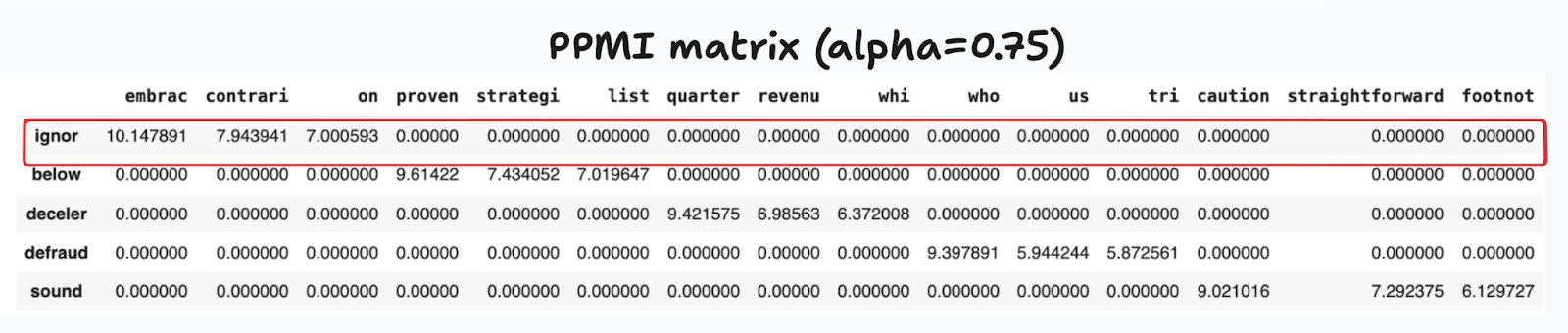
In these equations I have used a subscript ɑ to denote one common optimization done to this calculation. When ɑ=1, infrequent words have larger-than-expected PMIs. To address this bias, it’s common to use ɑ<1. In what follows I use ɑ=0.75 as proposed by Levi, et.al. (2015).2
Figure 10 shows the PPMI matrix for the term-term matrix presented earlier. For visualization purposes, I have chosen the top 5 words, each with its top 3 contextual words. As before, each row can be used as a word embedding.
Dense embeddings
With dense embeddings, we let machine learning algorithms calculate vectors for each word. Before the advent of LLMs, Word2vec and GloVe were the preferred alternatives to construct dense vector embeddings, and are still widely used to this day.3 I’ll first present the methods used to learn these embeddings, and then apply them to my dataset.
Word2vec & GloVe
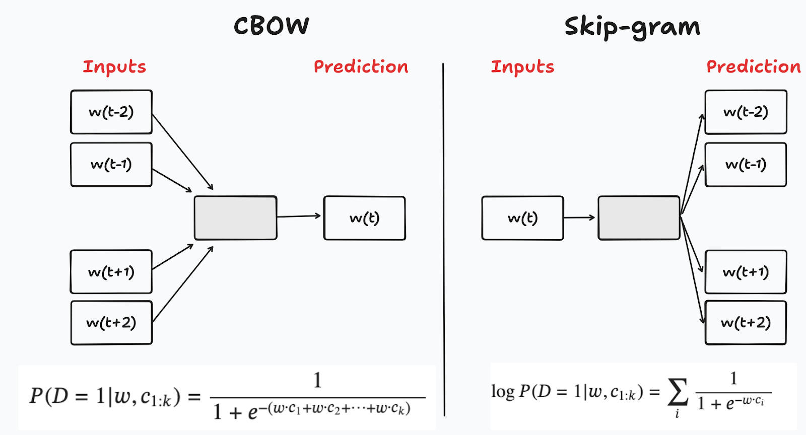
Word2vec uses two different methods to create embeddings: continuous bag-of-words (CBOW) and skip-gram. As with the term-term matrix, the idea is to consider a target word and the surrounding context. With CBOW, the objective is to predict the target word conditional on the context; the reverse procedure applies to skip-gram, where each of the target word is used to predict the words in the context (Figure 11).
These methods implement classification models where the objective is to predict if a given word-context pair (w,c) is in the corpus or not. The pairs in the training data are naturally used to create the positive dataset (D=1). The negative dataset is created by fixing a word and sampling pairs from the vocabulary (D=0). For instance, in skip-gram, for a given pair (w,c), you sample k target words w_k from the corpus (excluding w), to create k pairs (w_k,c). This method is called negative-sampling.4 Note also that to create a score, both methods use a similarity index that computes the inner product of the word and context word embeddings.
Global Vectors for Word Representation (GloVe) uses a slightly different approach to arrive at word embeddings. For each (w,c) pair in the term-term matrix (TT), the objective is to find embeddings that minimize the weighted sum of squared residuals between the observed frequencies in the term-term matrix and the dot product of the target and context words, respectively:
Figure 12 shows the first 10 elements (columns) for five words (rows) in the vocabulary created from the blog posts. I have used the models word2vec-google-news-300 and glove-twitter-25, trained with corpuses created from Google news and Twitter, with embeddings of sizes 300 and 25, respectively.

Dynamic embeddings
As discussed earlier, any LLM starts by transforming words into word embeddings.5 These learned embeddings are static, since the algorithm learns a fixed word embedding vector to each unique word in the vocabulary, independently of their context. Interestingly, many pre-trained LLMs also generate contextual embeddings, where a word’s representation depends on its context. The key insight is that the transformer architecture takes embeddings as inputs, and outputs a hidden state feature for each word in the training data. Moreover, thanks to the attention mechanism, these hidden states already take into account any cross-dependencies that arise for a given context window. Thus, these hidden states can be taken as contextual embeddings (Figure 13).

Let’s perform a simple experiment to understand the differences. Consider the next three sentences that use the word “run”:
S1 = "I am going to run a marathon."
S2 = "I am going to run for president."
S3 = "I am going to run a python script."
Since word embeddings are high dimensional, for visualization purposes it’s common to perform some type of dimensionality reduction technique. In Figure 14 I plot the first two principal components for the static and contextual embeddings for the word “run”, as obtained from BERT. Notice how the principal components for the first two sentences cluster together, suggesting that they are semantically more similar.

What’s next
In this first blog post on embeddings I wanted to present the different methods that can be used to construct word embeddings. Figure 14 highlighted one common application, where we assess the semantic similarity of different words. In the second part of the series I’ll explore this and other application in more detail.
In this post I refer exclusively to word or token embeddings, as opposed to positional and segment embeddings, commonly used in many large language models.
I’m following closely Ch.6 in Jurafsky and Martin (2023).
The 2013 paper that presented Word2vec won the Test of Time award in last year’s NeurIPS conference.
The authors of the paper also implement hierarchical softmax.
In practice, LLMs work at the token, or sub-word level, so embeddings also operate at that level.