The Importance of Feature Importance to Machine Learning Interpretability

Created with Dall-E 3

TL;DR

In this post, I discuss the importance of features for machine learning interpretability. I begin by arguing that data scientists start with some prior belief about the relative importance of the underlying factors of a model. Feature importance allows the data scientist to test their intuitions and the model at a high level very quickly, which is necessary for model improvement and debugging. I then simulate several models and showcase three alternative importance metrics: Shapley values, permutation-based importance, and impurity-based importance

Introduction

In a previous post, I described some of the most common methods used to understand the predictions made by black-box machine learning (ML).  One of the methods I mentioned in passing was feature importance, but I did not stop to explain how it works, or its relevance to the practice of data science.

Feature importance is a multifaceted concept, so in this post I start by discussing the different meanings and how they relate to each other.  This knowledge can help you in many day-to-day conversations with non-technical stakeholders, as these concepts are often easily misunderstood.

Feature importance metrics are commonly used as ex-post interpretability tools, but I’ve found that they correspond quite naturally with what I call ex-ante model design concepts.  In the latter, a data scientist starts with some prior knowledge about the underlying workings of a problem, including ideas about which variables matter most.  Contrasting ex-ante and ex-post importance allows the data scientists to iterate quickly and tell compelling stories.  

As usual, you can follow all of the calculations in the shared Colab notebook.

Storytelling-based feature engineering

Most of the time, when a data scientist starts working on a predictive model, they start by building a mental representation about the underlying factors that explain the given outcome.  In Data Science: The Hard Parts  (THP) I refer to this as ex-ante storytelling.  This is because the modeler creates stories that are refined by an iterative process, improving our own understanding of the problem and the predictive performance of the model.

For instance, if you’re trying to predict which customers are more likely to churn, you might start by stating that churn is the long-term absence of purchase intention, which itself depends on whether a customer wants or can make a purchase.  These factors can be modeled in terms of customer satisfaction at different levels, as well as other factors that affect their willingness to make a purchase (Figure 0). 

In THP I refer to these as the set of ideal features, since at this point, we abstract away any issues that may arise when we construct the actual features.  Once our understanding of the problem is in solid grounds, we can then consider whether these ideal features can be measured, or if they have to be proxied by variables that may affect one or several of the ideal features.

Figure 0: Ex-ante understanding of a prediction problem

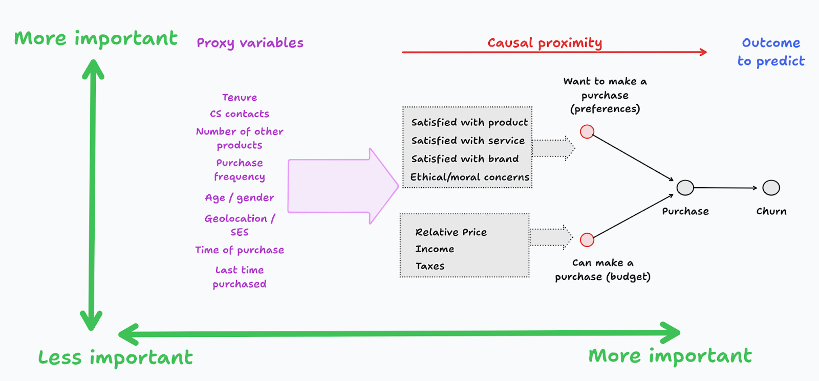
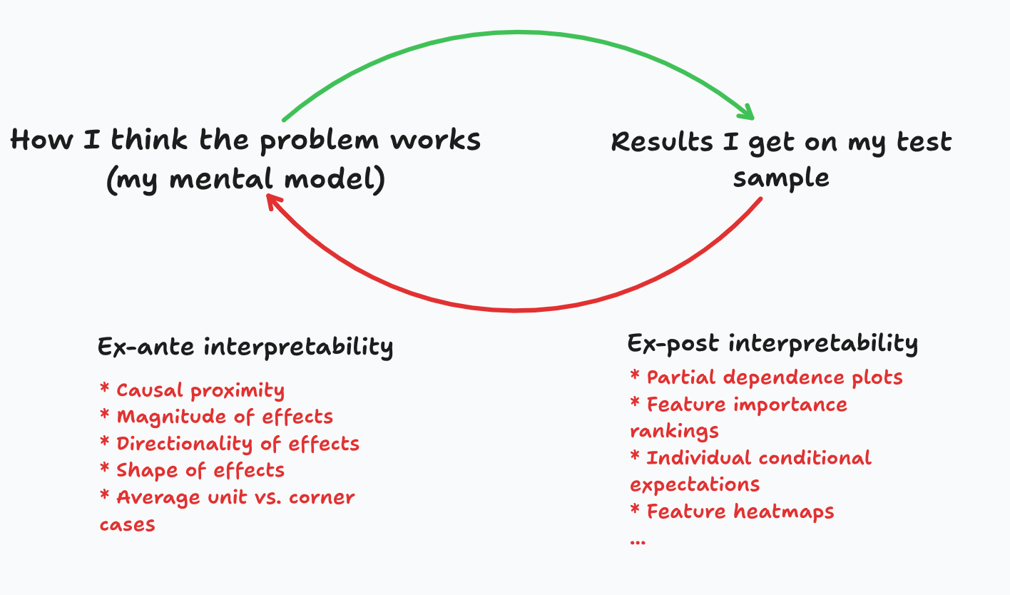
Figure 1 summarizes the difference between ex-ante design and ex-post interpretability.  Before coding an ML model, data scientists start with a mental model for the problem.  I always ask data scientists in my teams to formalize this, that is, to write it down, and present it to their colleagues, their manager, and even to myself.  Once the model is trained, they compute empirical interpretability metrics, and contrast them with their prior beliefs. 

Figure 1: Ex-ante vs. ex-post interpretability

Importance comes in many flavors

Exactly how this ideation process works varies from data scientist to data scientist.  In Analytical Skills for AI and Data Science I propose starting from factors that are of first-order importance and then move away to more distant ones.

But what do I mean by “distant”?  What makes a feature of first- or second-order importance?  Is it causal proximity?  Is it the impact on the outcome?  What about their individual impact on the predictive performance of the model?  The the top three dimensions of feature importance are presented in Figure 2, which I now discuss.

Figure 2: Different flavors for feature importance

Impact on the general prediction quality (loss)

Let’s start with feature importance in terms of the general quality of the prediction model.  Data scientists measure the predictive performance of their model with a loss function (L). Intuitively, if the predictions are perfect the loss is zero, so any deviations from this ideal increase the loss. One could imagine that different features affect the loss in different ways. Figure 3 shows one example, where the second feature appears to be more important, since its variation explains a larger chunk of the change of the loss function.  In contrast, the loss function is relatively flat with respect to x1.

Figure 3: Feature importance and impact on predictive performance

Impact on the actual prediction

Alternatively, we may measure relative importance in terms of the impact of a feature on the predicted outcome. Looking at Figure 4, x1 has a larger impact than x2 in, so in this view, we could say that x1 is more important than x2.  Naturally, this assumes that they are measured in the same units, so that an apple-to-apples comparison is possible.

Figure 4: Impact of each feature on an outcome

Causal proximity

As I described earlier, ideal features measure direct, or first-degree, causal relationships.  However, many times we need to be satisfied with using proxies that usually affect several direct features at the same time (Figure 5).  Interpretability for these more distant features tends to be substantially less crisp and transparent, but we live in an imperfect world, so data scientists are used to this handling this problem.

Figure 5: Causal proximity for feature importance

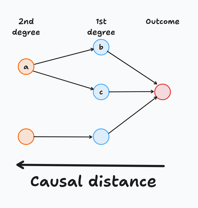
Intuitively, and other things equal, the closer the feature to the outcome, the more important it is.  For instance, in the figure, features b or c should be more important than feature a, but from this causal graph we can’t further rank them against each other.

Are these dimensions related?

If you remember from your ML 101 lesson, the loss function measures the average predictive performance of the algorithm, which depends on the trained prediction function.  For regression models, a Mean Squared Error (MSE) loss function is commonly used, and for classification a log loss or cross-entropy is quite standard:  

\(\begin{eqnarray} L(y,f(x)) &=&  \begin{cases} \frac{1}{n}\sum_{i=1}^n (y_i - f(\mathbf{x}_i))^2 \\ \frac{1}{n} \sum_{i=1}^n y_i \log(p_i(\mathbf{x})) + (1-y_i)\log(1-p_i(\mathbf{x})) \end{cases} \end{eqnarray}\)

Naturally, if a feature impacts the prediction it will also impact the loss function (Figure 6).  Taking the absolute value, you can see that these two measures are proportional to each other.  This correlation will be apparent later when we explore some empirical metrics of importance.  

Figure 6: Loss and prediction function are closely related

Note that one can derive a similar expression for causal proximity, and track the impact that any individual feature may have on the outcome and the loss. Distant features tend to be noisy with respect to the outcome, thus diminishing our ability to separate signal from noise.¹

Note also that if we are able to “control” for the more direct causes, distant features should have a negligible impact on the outcome and the loss function.  The Frisch-Waugh-Lovell theorem  guarantees that this is the case in linear regression, but it may not apply with ensemble-based algorithms.²

Empirical measures of feature importance

I’ll discuss now the most common feature importance metrics, starting first with linear regression, the baseline that I always used when discussing interpretability.

Linear regression to gain some intuition

Let’s start with linear regression, to set a benchmark and to gain some intuition.  In a regression model, the parameters and the variance of each feature play closely related roles, as can be seen from the next equations:

Equation (1) is a standard linear model with three features, and equation (2) is a model where the outcome and the features have all been standardized, so everything is measured in units of standard deviations (so a better word is “unitless”).  By replacing the definition of prime variables in (2), we can see that the two sets of parameters are closely related by a proportionality factor:

Let’s start by simulating two simple models:

• M1: all features drawn from a standard Normal distribution, and have unit slope parameters.

• M2: same as M1, except that x3 is drawn from a normal distribution with mean and variance parameters given by N(0,4).

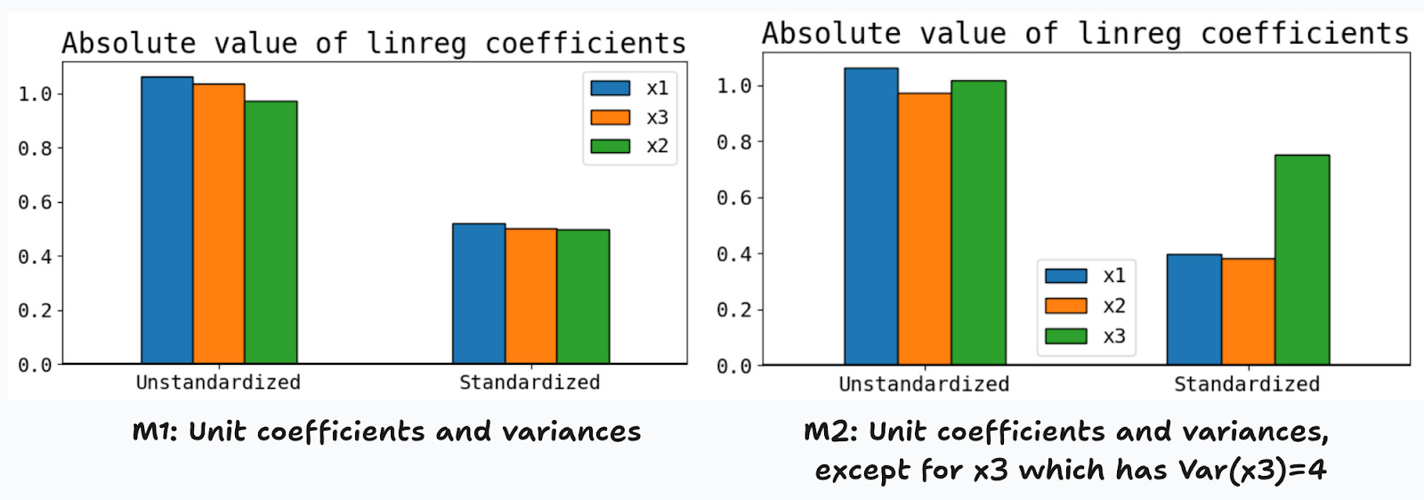
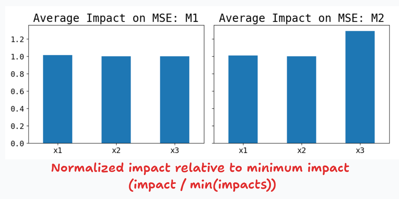
What should we expect in terms of feature importance?  Since M1 is completely symmetric, any reasonable measure of importance should allow us to conclude that all features are equally important.  For M2, thanks to the proportionality factor above, it’s natural to expect that the third feature is found to be twice as important as the other two, themselves being equally important.

If true, these intuitions will lead us to conclude that in standardized linear models, the absolute value of the parameters are a reasonable measure of feature importance.  Figure 7 shows that this is indeed the case.  For M1, we find no significant differences in the estimated coefficients of standardized and unstandardized features (left panel).  For M2, once we standardize the features, the coefficients rank the features as expected, and the third feature is now twice as important as the first two.

Figure 7: Feature importance with linear regression

Let’s explore the impact on predictive performance now.  Figure 8 shows that increasing the variance by 4x, has an impact on the MSE of around 29%.  This metric of feature importance is directionally correct, but higher variances don’t translate one-to-one to changes in predictive importance.

Figure 8: Normalized MSE feature importance for models M1 and M2

General metrics for feature performance

The three most common metrics for feature performance are (1) permutation-based, (2) impurity based, and (3) based on Shapley values.

I described Shapley values before, so I will now show how permutation- and impurity-based metrics work.

Permutation-based importance

Permutation-based importance was first proposed by Leo Breiman in the paper where he introduced random forests.  The idea is relatively simple, and can be performed using these steps:

1. Base loss: fix all features at the current values, and calculate and save the base loss evaluated using the test sample.

2. Permutation: for the feature of interest, shuffle or permute their values across units.

3. Predicting: using these new features, make a prediction and record the loss function.

4. Relative impact: measure the relative impact against the base loss

5. Repeat: repeat steps 1-4 many times and average out the relative impacts.

From step (4) you can see that permutation-based importance measures the relative relevance in terms of predictive performance.  Put differently, a feature is more important whenever the relative impact on the loss is larger, in absolute value terms.

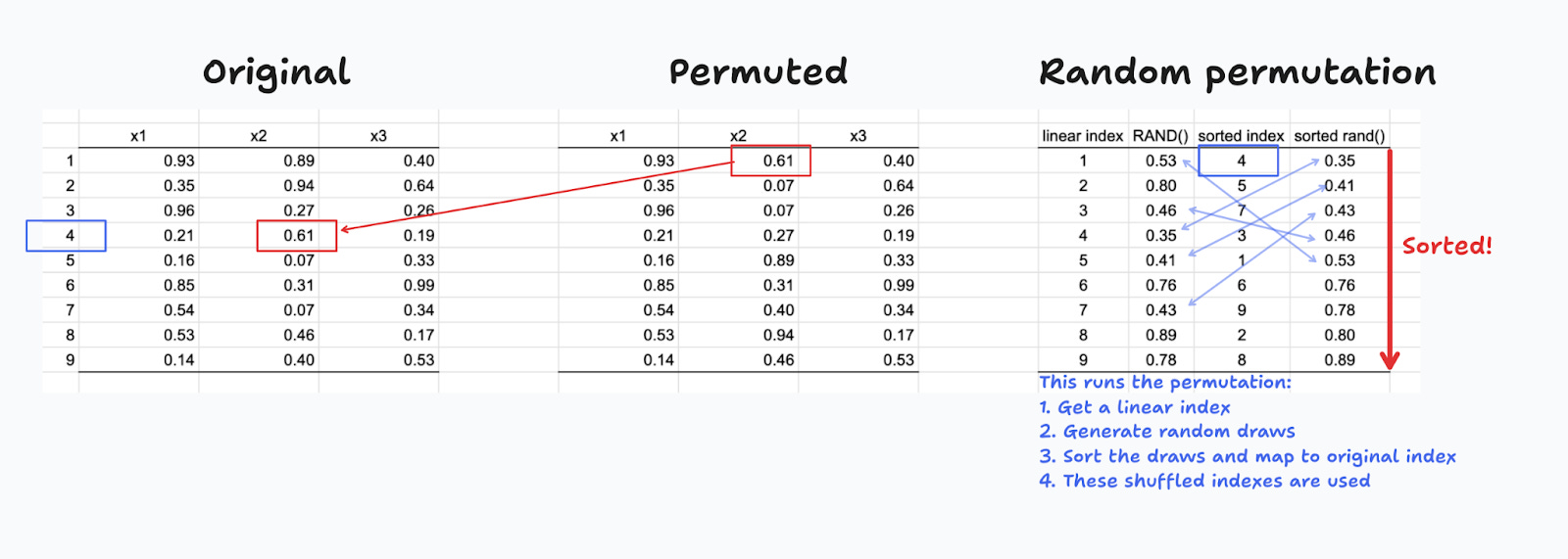
Figure 9 shows how this can be implemented in practice.  Here, I want to get one random permutation of x2.  I first create a linear index (rightmost table), and then make random draws for each row in the table.  I then sort these draws in ascending order, which has the effect of providing of also shuffling the linear index. The latter is used to find the corresponding shuffled values for x2.

Figure 9: Random permutation

Why does this work?  Consider a feature z that you decide to include in your model, but has no explanatory power.  If you shuffle its values, the predictive performance of the model should not change, so z should have zero relative impact on performance.  For features that have explanatory power, the impact on the loss depends on the relative sensitivities of the loss function and the prediction function. as explained above.

Alternatively, compare this approach to how Shapley values are calculated(Figure 10).  With Shapley values, the incremental impact of a feature is estimated by looking first looking at any combination of features that contain it, dropping it, and calculating the impact.  “Dropping” a feature is implemented by drawn from the empirical distribution many times, and averagin out the effects.

Before moving on, note that with permutation-based importance it’s quite standard to also report the confidence intervals since we are effectively bootstrapping the results.³ In the results below I will be reporting 90% confidence intervals.

Impurity-based importance

Tree-based algorithms, such as Classification and Regression Trees (CART), along with ensemble methods like Random Forests and Gradient Boosting, have their own methods for assessing importance.  

Recall that when growing a single binary regression tree, you first split the root node by testing all features and threshold values, and choose the feature with the highest improvement in MSE (in Figure 10 we choose x1 first, with a threshold of 10).  This process continues until the the maximum depth of the tree is reached.  The actual implementation of the algorithm saves each of the relative MSE improvements from the best splits, for each feature, across all nodes, so for a single regression tree the total relative improvement for each feature can be easily computed.  Moving from individual trees to tree-based ensembles is relatively straighforward, since you just need to compute the sample average across all trees in the ensemble.⁴

Figure 10: Growing a binary tree

The word “impurity” comes from the fact that, in classification settings, different impurity measures åre used to split each node.  Typical impurity metrics are the misclassification error, Gini index, or the cross-entropy (or deviance).  Other than this, the algorithm works the same as with regression: you test all features and thresholds first, and choose the optimal by computing the relative impact on predictive performance, as measured by the chosen impurity metric.

Note that permutation- and impurity-based metrics both rank the relative importance of features with respect to their predictive power, not the impact on the predicted value.  This is in contrast with Shapley values importance, that are computed by averaging out the absolute value of individual Shapley contributions on the actual prediction.

Simulations

To test and compare each of these methods, I’ll simulate four linear regression models with three features (Figure 11).  The first two models are the same as before:

• Model 0: unit slope parameters (in absolute value), and each feature is drawn from a standard Normal distribution.  

• Model 1: same as Model 1, but x3 is drawn from N(0,4)

• Model 2: x2 affects x3, but has no effect on the outcome.  Good to test for causal proximity importance.

• Model 3: x2 affects x3 and the outcome (direct and indirect effects)

Figure 11: Simulated models

To compute the three feature importance metrics (permutation, impurity and Shapley), I first train gradient boosting regressors (with metaparameter optimization) and then use these models to compute the metrics.

Figure 12 presents the results which I now summarize:

1. Consistency across estimators: The three metrics give results that are consistent with each other.  

2. Consistency with ex-ante intuitions: symmetric features have similar importances (Model 0), features with higher variance provide more information and are thus more important (Model 1), inconsequential features have no importance (Model 2).

Figure 12: Different feature importance for each of the simulated models

Results are less straightforward for Model 3.  On the one hand, since x3 depends on x2, it also must have a larger variance, which translates to higher feature importance (as Model 1 showed).  The results are consistent with this intuition. However, x1 and x2 should have the same importance, which is not happening.  I don’t have a definite answer here, but here’s my intuition. 

First, I used the default tree depth (max_depth = 3), and optimized only the number of trees (n_estimators) and the learning rate.  Since x3 depends on x2, it already captures some of its variation, and when the trees are grown, once they stop choosing x3, the algorithm switches to selecting x1 instead of x2.  But trees reach quickly the maximum depth allowed.

What next

Feature importance is the first interpretability metric that should be reported, only after showing that the model actually does a good job at making predictions. Findings that are not consistent with your prior beliefs may signal problems in how features were coded, or even the presence of data leakage. Understanding how each importance metric is calculated, as well as the intricacies of the predictive algorithm, is critical to assess if the model is sensible and can thus be deployed to production, or if further iterations have to be done.

1. In Chapter 9 of THP I discuss signal-to-noise considerations.

2. In Chapter 10 of THP I discuss the Frisch-Waugh-Lovel theorem and show examples where uninformative features appear to be informative just because of the algorithm used.

3. I cover bootstrapping in Chapter 9 of STP.

4. A good reference is Hastie, et.al., “The Elements of Statistical Learning”.  See page 387.