


Word Embeddings Applications: Part 2


TL;DR
Word embeddings lie at the heart of many generative AI (GenAI) applications. In Part 1 of this series, I showed how to construct word embeddings, starting from sparse embeddings that use the term-document and term-term matrices, or their weighted versions using TF-IDF and PMI, and going into learned dense embeddings that include static and contextual embeddings. This post is all about applications, so you can follow all of the calculations in this Google Colab notebook. I will start by showing how word embeddings enable you to quantify the semantic distance of words. I will then move to methods to find sentence and document embeddings, and finally I’ll apply these methods to a dataset consisting of the posts I’ve written on Substack and chapters from one of my books.
Similarity
Just as a reminder, word embeddings transform words that live in the lexical space, into real-valued vectors of dimension d. This transformation is quite useful, as we can define distance functions on real numbers and vectors, which can in turn be used to assess similarity between words. For instance, assuming that embeddings are good at capturing the meaning of words, we should be able to conclude that the words “model” and “prediction” are more similar to each other than to the word “house”. Once we tackle semantic similarity, we can also do tasks like finding analogies (Figure 1).

With word embeddings, it’s quite common to use cosine similarity:
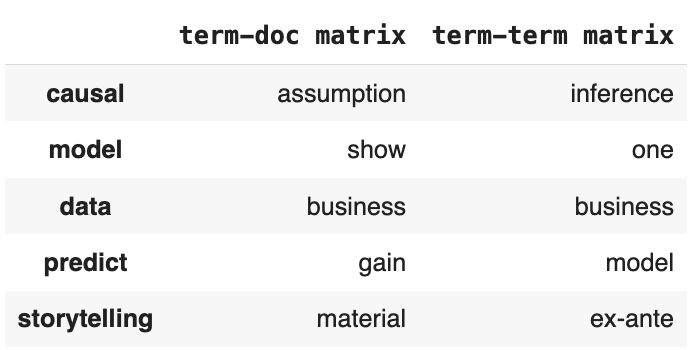
It can then be used to find a word that is most similar to another. Figure 2 shows the words, among those used in previous blog posts, that are most similar to “causal”, “model”, “data”, “predict” and “storytelling”, using the embeddings calculated from term-doc and term-term matrices described in Part 1.
From word embeddings to sentence and document embeddings
One natural question that arises very quickly is how to move from words to sentences, paragraphs or even documents. To be sure, in today’s practice, we start by tokenizing words, so learned embeddings operate at this subword level. Nonetheless, from now on I will use these words as synonymous, and refer only to words.1
Most applications require us to perform information retrieval at the document level, so there has been quite a bit of research around the problem of generating embeddings at the sentence or document embedding. I won’t go into the earlier literature, but I’ll start with Devlin, et al., (2019)’s paper that introduced BERT (Bidirectional Encoder Representations from Transformers) that had a deep impact on the current practice.
At a very high level, BERT converts words into static embeddings, which then go through several transformer blocks or layers, and for each word in the training data set it generates one hidden output (Figure 3). Another important feature is that sentences are separated with special characters: [CLS] is included at the beginning of every sentence, and there’s another special character [SEP] used to separate questions from answers. The [CLS] character plays an important role in what follows.2
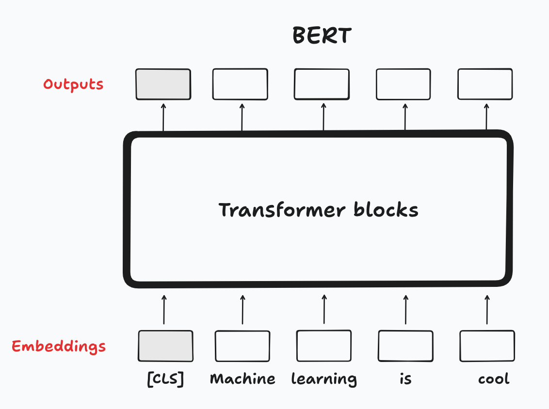
As was discussed in Part 1, the embeddings at the base of the LLM are static, since they map one-to-on to words in the vocabulary. However, the outputs at the top are contextual embeddings since they map each word in a sentence to vectors (of the same size H as their static counterparts), and they have gone through the transformer blocks that provide information about the context for each word. When computing sentence and document embeddings we work with these contextual embeddings.
Take the sentence “Machine learning is cool!”. To get contextual word embeddings you first include the [CLS] token and then compute a forward-pass on each word, to generate contextual embeddings (Figure 4). To get an embedding for the sentence there are generally two approaches:
[CLS] token: use the embedding of the [CLS] special token as the embedding for the whole sentence.
Pooling: Perform some type of pooling or aggregation, such as averaging the embeddings of each word. An alternative pooling strategy is to compute the maximum across embeddings. Note that these preserve the dimension of the output vectors, since it’s an elementwise operation.

To recap, in this approach you start with a pre-trained model like BERT, generate word-level contextual embeddings for each of the sentences you want to embed. You can use the [CLS] token if you’re using a BERT-like model, or average across word embeddings.
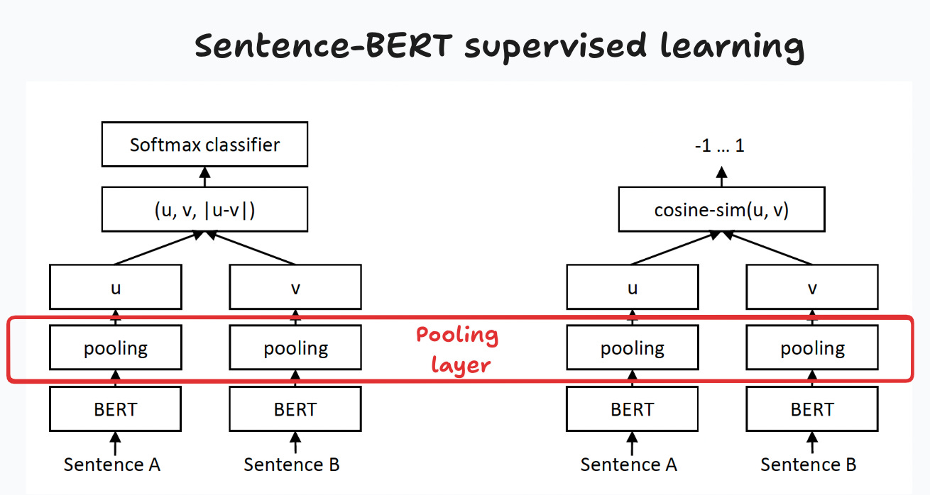
As usual, one can further improve the performance of the embeddings by performing some form of supervised fine-tuning. This is the approach taken by Reimers and Gurevych (2019), “Sentence-BERT: Sentence Embeddings using Siamese BERT-Networks”. They fine-tune two siamese BERT networks to get embeddings that capture the semantic content of the sentences.3
Figure 5 shows the two supervised learning objectives they use for their fine-tuning task. They use the SNLI dataset, consisting of 570K sentence pairs, each labeled as entailment, contradiction, or neutral.4 First, they pool word embeddings, using one of the three strategies described previously ([CLS], mean-, or max- pooling). These embeddings are then passed through one of the two objective functions. Their main finding is that this method outperforms pooling on the pre-trained BERT and GloVE, and importantly, they open sourced the fine-tuned models for our use.5
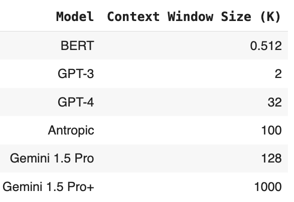
What about embedding entire documents? First, recall that transformers are restricted by a context window that determines how far into the “past” (self-attention) or “future” (bidirectional self-attention) the model is allowed to explore for each word. For instance, BERT uses a 512 tokens combined context size window that spans the left and right of each word. Table 1 shows context window sizes for different LLMs.
The previous method — sentence-transformers — can be applied to larger documents that span several sentences, but always under the restriction that it’s length is not longer than the context window. For instance, if you have a document with more than 380 words, say 600, it will chunk the document into two parts that can then be fed into the model. It will then compute the embeddings for each of these documents, which can then be pooled to find the embedding of the model. Note that sentence-transformers uses the full extent of the context window when computing the embeddings. For instance, if you have a document with two sentences like “I want to embed a document with two sentences. How should I proceed?”, since the length of the document fits the context window, it will directly find the embedding for the whole document, instead of splitting it into sentences and pooling the results.
Applications
I’ll start by using the word2vec embeddings introduced in Part 1, and show how you can extract the semantic content of words. To visualize the results I’ll use the following approach:
Dimensionality reduction: I first reduce the dimensionality of the word embeddings (of size d=300, since I’m using
GoogleNews-vectors-negative300). For this I use TSNE or UMAP, but you can use any other dimensionality reduction algorithm, like PCA.Clustering: I then try to extract clusters using HDBSCAN.
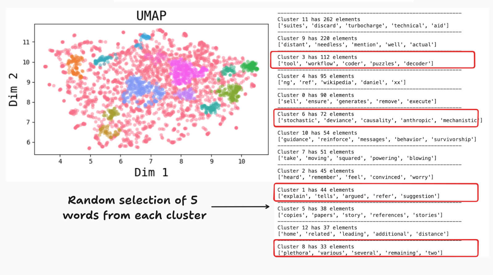
Figure 6 shows a typical visualization of the two dimensions extracted by UMAP, and the 12 colored clusters found with HDBSCAN.6 The vast majority of words (in pink) are assigned to cluster -1, which HDBSCAN uses as a default or residual cluster for noisy words. On the right I show 5 sampled words from each of the clusters, that help with with interpreting each cluster. For instance, clusters 3 and 6 include some programming and technical words. Cluster 4 finds some proper names and acronyms, and cluster 0 appears to group verbs.
I now move to document similarity, and compare Substack posts and each of the chapters of Data Science: The Hard Parts. On Substack I’ve expanded on topics discussed in the book, so I should be able to find the chapter that is most similar to each blog entry. To do this I first embed the chapters and blog posts, and then compute cosine similarities to find the most similar chapter for each blog post. The results are presented in Figure 7. For instance, the blog posts on confounder bias and causality and decision making are extensions of Chapter 15 Incrementality, and the post on ML and decision making is also closely related to incrementality. The results make sense, but to get more robust results I’d need to do more tweaking. I’ll cover some of the intricacies of this “tweaking” in a future post on Retrieval Augmented Generation (RAG).

As a final application, let’s use BERTopic to find some clusters for the set of documents. As before, BERTopic starts by embedding each document, reducing its dimensionality and performing some type of clustering of these reduced embeddings. To facilitate the interpretation of each cluster we use class a class-based TF-IDF method, which adapts the document-based TF-IDF presented in Part 1 to take care of clusters (or “classes”) of documents. The idea is that the most important terms, according to c-TF-IDF, will provide an interpretable labeling for each cluster.
Figure 8 shows the results. As before, I may want to do more tweaking of the different components to get more informative results, but this is good enough for the purpose of this post.

Other applications
There are many applications that are enabled once you realize that embeddings give you the power to use distance or similarity functions over language. You can use topic modeling to classify documents or interactions with your customers, or do anomaly detection over texts to enable the content moderation service for your website. You can elso enrich search and retrieval. Imagine searching for a product on Amazon, or for a place to stay on Airbnb, where you just say, in plain English, exactly what you’re looking for. I will devote a future blog post on the topic of RAG that powers many of these applications.
When thinking about tokens, it’s good to use the rule of thumb that one token corresponds to roughly 0.75 words.
Note that BERT also includes positional and sentence embeddings. As the word suggests, positional embeddings provide a sense of where the word is in a sequence, and sentence embeddings help the model identify different sentences.
Siamese networks share their full set of parameters, reducing the computational cost when fine-tuning.
An example of sentence entailment are the sentences "Pat is a fluffy cat" and "Pat is a cat". The first entails the second one, since if the first is true, the second one is also true.
You can access them through their website, or through the Hugging Face sentence-transformer API.
Extracting meaningful clusters is rarely accomplished immediately, and it usually requires quite a bit of testing. You can check the notebook and see several of these trials.