
What is Confounding or Selection Bias?


In a previous post, I discussed confounder bias in the context of causal directed acyclic graphs (DAGs) and highlighted its relevance for data-driven decision-making. In this post, I aim to delve deeper, demonstrating how it can potentially impede causal inference.
Confounders: an example
In Analytical Skills for AI and Data Science I motivated this discussion by trying to answer the question: “are doctors incremental to your health?” Suppose that the People team wants to evaluate the incrementality of providing health insurance to the employees. To do so, six months after launch, they conducted a survey among all employees, asking them to rank their health status from 1 to 5 (5 being the highest). Their data scientist suggests computing a difference in mean health status between those who used it (u) and those who did not (d):
Figure 0 shows the average self-reported health status for the two groups, along with 95% confidence intervals. The results took the HR team by surprise, as they indicate that providing insurance actually worsened the health of the employees! But is it really?

Welcome confounders: DAG
These results are so counterintuitive, that the natural instinct for the data scientist is to delve deeper into the problem. Figure 1 shows a DAG drawn for this problem. Just as a reminder, a DAG is a set of nodes (variables) that may be connected through causal relationships (arrows). Importantly, this is our model of how the variables affect each other, that is, it describes a set of assumptions about how we believe the problem works.
In this case, (i) I assume that going to the doctor (using the insurance) effectively affects an employee’s health status. Moreover, I expect this to be a positive effect, but that DAG can’t represent this, it only displays causal relationships. (ii) Naturally, if I feel sick, I will also self-report a lower health status. Finally, and importantly, (iii) those who feel sick actually use their insurance.

Notice how feeling sick affects the two other variables, and thus it acts as a confounder for the actual causal impact we care about (insurance → health status).
Confounders and selection bias
Among causal inference scholars and practitioners there are two schools of thought: the DAG and the potential outcomes (PO) teams. I won’t discuss now how the second approach works, but if you’re interested you can read chapter 15 of Data Science: The Hard Parts (THP). What matters is that confounder and selection bias are two names, given by each school of thought, for exactly the problem described above.
Being an economist trained using the PO approach, I prefer thinking about behavior rather than the more mechanistic DAG approach. For instance, in this example, the employee decides to use their health insurance because they feel sick. Put differently, there’s some possibly unobserved variable (feeling sick) that makes them self-select into going to the doctor. I’ve found that whenever an analysis deals with human subjects (e.g. customers) it’s always better to think in terms of behavior and incentives, which maps quite naturally to the powerful concept of self-selection and selection bias.
If you want to think more mechanistically or algorithmically, you can draw a DAG and check all variables to see which ones act as confounders for others. This approach is more prone to automation, so naturally it has found more adherents among computer scientists. But even if you use this approach, you have to think hard about causal relationships (which nodes are connected by arrows and why) and proceed to model them.
The key takeaway is that selection bias is confounder bias (and vice-versa).
Self-selection and selection bias
Self-selection and selection bias are two sides of the same coin: with self-selection, the decision maker opts for the treatment — in the example, visiting the doctor — whereas with the broader concept selection bias, the decision could be made by the individual in question or by someone else.
In the example, I self-select into going to the doctor only if I feel sufficiently sick (otherwise, I’d prefer to engage in a different activity).
In THP, I also discuss the case of adverse selection where, for instance, predominantly high-risk users accept loans with high interest rates. This scenario frequently arises in numerous use cases across the fintech sector.
Often, it’s you, the company, that makes a selection. In THP, I also discuss a common problem that arises when evaluating the effectiveness of marketing campaigns, as the team frequently preselects the target audience. This selection typically comes in the form of filters or rules such as “include customers who have been active for at least 6 months, made a minimum of 10 purchases in the last 12 months, and reside in the Northeast region.” All these filters create a selection bias that needs to be taken into account.
Selection and survivorship bias
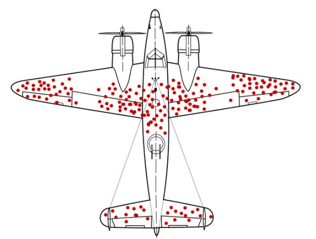
Most data scientists learn about survivorship bias through Abraham Wald’s recommendation to reinforce those parts of the military aircrafts that had not been hit during WWII (Figure 2).
Survivorship bias is studied as a cautionary tale, emphasizing the critical importance of understanding the sampling process for one’s data. Let’s apply this to a common use case found in many companies. Suppose you want to know whether your customers like your product. It’s common practice to send online surveys asking them if they would recommend your product, using a scale from 0 to 10. You can then compute the Net Promoter Score.
The problem is that customers usually self-select into answering the survey. Can you really infer anything about the overall customer base, or are you primarily capturing the preferences of the most dissatisfied customers? Those customers who respond to the survey have survived the sampling process by opting to provide feedback. In this regard, selection and survivorship bias are two sides for the same coin.
Dealing with confounder bias
Ok, you have figured out that selection or confounder bias might be important for your analysis, then what? The answer to this question depends critically on whether you observe or not the confounders. The PO school calls this selection on observables, since it’s required that you observe all variables affecting the probability of entering into the treatment (selection).
If you don’t observe all confounders, you can’t move forward. There’s no way you can credibly estimate the causal effect. This is why causal inference is so hard: you not only need to have the correct model of the world (your DAG), but you also need to observe all possible confounders.
If you do observe the confounder (Z) there are many things you can do. The most common is using linear regression:
By regressing the outcome (y) on the treatment (D) and the confounder (Z) you effectively eliminate any confounder bias from the treatment effect.1 The estimated coefficient (beta) is your causal effect, which you can report or plot as before.
Alternatively, you can also match your customers using the confounder, and compute the difference for different Z-segments and then average these out. For simplicity, suppose that Z can only take three values 1,2,3 (1: I feel great, 2: I feel somewhat sick, 3: I feel very sick). If there is overlap, for each of these segments (z) you can compute:
Note that there has to be some overlap, otherwise there might be segments where you only observe one of the two groups, and thus, you won’t be able to compute the corresponding difference.
This simplified “matching” estimator can be generalized to the actual matching estimator where each subject in the treatment group is matched to a group of subjects in the control group.2
What next
By now, I hope I have convinced you that causal inference plays a critical role in data-driven decision-making (and thus in data science), and that a solid understanding of confounder or selection bias can take you very far in estimating and disentangling causal effects. However, this is not to suggest that confounder bias is all you need to learn; the field of causal inference is extensive (and fascinating).
This is thanks to the Frisch-Waugh-Lovell theorem. See chapter 10 of THP.
I describe matching and propensity score matching in chapter 15 of THP.