


Opening the Black Box: The Role of Interpretability in Machine Learning


TL;DR
While many machine learning (ML) models boast high predictive performance, they often fall short in offering clear explanations for their predictions and the overall prediction process. Interpretable ML, a set of tools and methods designed to open the black box, is a crucial skill set for any data scientist working in ML. Interpretable ML not only aids in improving existing models and deepening our understanding of the problem at hand, but it may also be required for regulatory compliance. Moreover, it can enhance your storytelling abilities. In this post, I will demonstrate how some of these methods work, including feature heatmaps, partial dependence plots, individual conditional expectations, and Shapley values.
Introduction
The success that data science experienced in the last decade and a half is partly explained by having more data, open source technologies that lowered the barrier of entry to a highly specialized and technical field, cloud technologies and compute and hosting availability, and having more powerful predictive models.
These models are highly nonlinear, they take care of any interactions between features without human intervention, and if you use some type of regularization method, they can also take care of eliminating features that have lower explanatory power. In this sense, the data scientist “just” chooses a set of variables that go into a black box, which almost magically comes up with superior predictions (Figure 0).

The subfield of machine learning (ML) interpretability emerged to enable the opening of these black boxes. In this post I discuss its relevance to the practice of data science, and showcase how some of the methods work in a highly controlled environment that facilitates the understanding. This discussion is a good complement to Chapter 13 of Data Science: The Hard Parts (THP), but it can also be read independently. The code used can be found in this Colab notebook.
Interpretability defined: motivating example
A data scientist working with a drone delivery company, wants to predict the time it takes an object to reach the ground when dropped from different heights and different locations around the globe. She has a rich dataset for many experiments run across the globe. After careful consideration she decides to use the following features to predict time:
Height (ℎ)
Initial velocity (𝑣)
Mass (𝑚)
Distance of each location to the Equator (𝑑)
Her abstract mental model is thus something like:
From previous experience, she decides to use a black-box algorithm (e.g. an ensemble model, like random forest or gradient boosting regression). The results are good, but in some cases are somewhat counterintuitive.
This is a rather typical way for many data scientists to pose problems.1 Ideally, an ML algorithm will both be predictive and interpretable. Linear regressions and decision trees are examples of highly interpretable algorithms, but lack in predictive power. On the other extreme are models with high predictive power and low interpretability, such as deep neural networks – like those powering generative AI applications –, support vector machines, or gradient boosting regression and classification.
The ideal algorithm will both be predictive and interpretable
Local vs. global interpretability
Broadly speaking, an algorithm is interpretable if we can understand the process by which it makes predictions, both at an individual or unit level, and in a more general sense. These are known as local and global interpretability, respectively.
In the example, it would be great if we learn that the mass and distance to the Equator play no role in explaining the time it takes after dropping the object. Even better if we could also recover the true underlying data generating process (DGP), so that we learn that the height is a nonlinear function of the initial velocity and the time it takes to reach the ground, and a quadratic function of time (se we can then solve for time and use it as the outcome in our model):
These are all cases of global interpretability. On the other hand, if we want to understand how a specific prediction came about, we are in the realm of local interpretability.
Using feature variation to interpret models
One key principle in model interpretability is that we can use the model, along with controlled variation in one or several features, to gain insights into the underlying workings of the model.
In the previous example, suppose we allow time to vary, but fix every other feature at its average sample value. We can then simulate height as a function of time, and time only, and find that our gradient boosting regression recovered the quadratic nature of time of the true DGP (Figure 1). Note that “simulation” here really means “prediction” but the data scientist decides which features vary and which don’t.

What matters at this point is that if we have enough variation in our features, and a model to predict, we can gain some insights about the underlying workings of the model.
Why is interpretability important?
Why should we concern ourselves with interpretability, when our primary focus is on predictive performance? This is a fair question, so let’s address it now.
Regulation
Opening the black box is often required for regulatory purposes. For instance, many companies in the US and the European Community are required by law to provide the reasons for a specific credit application denial.
Fairness
Models are used to make decisions, and these decisions can have a huge impact on our lives. For instance, you could be denied credit or parole for reasons unrelated to your ability to repay a loan or your actual likelihood of reoffending, such as your skin color. The field of fairness in ML has become of critical importance for use cases that explore the fairness of an ML-driven decision.2
Understanding
You may simply wish to understand the workings of the model, or verify if the predictions align with your intuitions. While this could be driven by pure intellectual curiosity, it could also help you secure buy-in from your internal stakeholders. It’s easier to persuade your audience if they understand and the results are consistent with their intuitions.3
Whenever a data scientist is presenting the results of a model, I always ask them to start by showing some performance metrics, and then some minimal interpretability results. I may ask them to go back to the drawing board if these two first quality checks don’t meet the required standards.
Model improvement
In THP I show how you can use interpretability methods to improve your ML model. For instance, the first question you should always ask as a data scientist – from anything from a query, a transformation, a visualization or a model— is whether the results make sense. Usually this helps you iterate on your feature engineering process and improve on the predictive performance of the model.
Interpretable ML can be very useful to check if your results make sense.
Similarly, this can be used to debug your model. A common and challenging type of bug arises from logical errors, where a mistake has been made in the computation, but your code runs without errors. The methods available in the interpretability toolkit can assist you in finding these errors. Finally, understanding your model predictions can aid in identifying and fixing any sources of data leakage.
Storytelling
In THP I also show how these methods can help you with your end-to-end storytelling. Stakeholders are less likely to block you from deploying the model into production, if you can tell them stories that are deeply connected to the underlying workings of the business. Some of these stories are surprising and create memorable Aha! moments, and others will align nicely with any preconceptions they already have.
Improved decision-making
One topic I explore in the last chapter of Analytical Skills for AI and Data Science (AS) is using predictions to directly impact a metric. Suppose that you have a model like:
where the objective is to predict a metric (m) when some exogenous features take some values (xk) and you can choose the level of the specific lever. Exogenous features are not under your control, like the weather, and a lever is always under your control, by definition. If you have such a reliable prediction model, you can then choose your lever to improve on your metric. Later I’ll provide a concrete example.
Some methods for interpretability
Let’s delve into the actual methods. For today’s purposes, I will simulate a dataset for a loan default prediction model tailored for small and medium businesses (SMBs). The advantage of simulating the data is that it allows me to control every aspect of the true DGP, enabling me to test the results using various interpretability methods against the ground truth.
I first simulate a simple-enough model that captures the following intuitions, which are further explored in the shared Colab notebook:4
Fraud motive: Newer customers are more likely to default.
Reciprocation motive: Angry customers are more likely to default. I proxy “angriness” with the number of contacts per month.
Financial conditions motive: SMBs that are growing faster are less likely to default. I use the change in revenue in the period right before the loan application.
Adverse selection motive: SMBs that take loans with relatively high interest rates are more likely to default.
Naturally, in a real-life application, you would expand on these hypotheses, but this simple model is minimal enough to showcase several interpretability methods. In what follows I’ll show the results of trying to predict which SMBs default, using an out-of-the-box gradient boosting classifier, but the underlying logic applies to most other classification or regression models.
Before moving on, notice that the last hypothesis includes a lever as a feature (interest rate). If the model is predictive enough, you can use it to customize rates to different customers.5
Feature heatmaps
Feature heatmaps are not commonly described in interpretability textbooks6, but the technique is so easy to implement that I always ask data scientists in my teams to present them.
To compute the heatmap you follow the next steps:
Make a prediction for your test data. Use your model to make a prediction for each unit in your data. In this example we’ll get a predicted probability score for each SMB.
Calculate scores deciles. Sort the probability scores, and split the sample into equally sized buckets, say deciles.
Calculate average values for each feature. For each feature and bucket, calculate the average value of the feature for units in that bucket, and save it on a table.
Plot: Plot these data on the table using a heatmap.
The idea is quite simple. You have a classifier that predicts a probability score that an SMB will default or not. Ideally, your score is informative in the sense that higher predicted probabilities are associated with higher default rates. Fortunately, this can, and should always, be checked first. Figure 2 shows the heatmap for the simulated example.
Feature heatmaps are a quick method to check if the results make sense from a directional point of view.
Feature heatmaps are read from left to right, starting with the top features and continuing downwards. On the vertical axis, features are most commonly sorted using some measure of feature importance, to ensure that you start interpreting the most relevant ones. The color shades and the labels quickly show the presence or absence of any correlation between the values of the feature and the score. For instance, you can quickly check that SMBs that had lower revenue growth are more likely to default.
Wouldn’t it be great if you could conclude that increasing interest rates 11pp, increases default from 0% to 58%? It would be great, but you can’t say this from a heatmap. Heatmaps, as well as all other methods in the interpretability toolkit say nothing about causation. Furthermore, while it’s true that your model sorts correctly across buckets, in the sense default rates increase from 0% to 58%, you can’t say which feature is most responsible for that increase.

Caution! Methods for interpretability won’t allow you to conclude anything about causation.
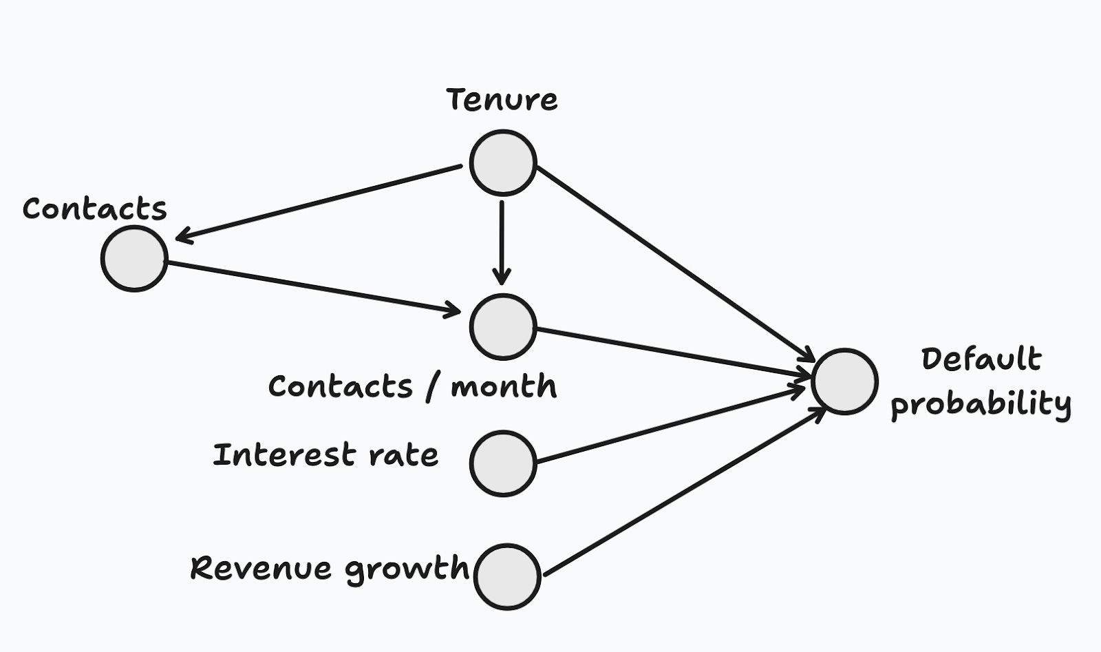
Heatmaps are a simple tool to quickly check global interpretability, but simplicity comes at the expense of reliability. For instance, I included the total number of contacts to customer support (CS contacts) on purpose, but it does not affect the default probability (I know this because I simulated the model), and it’s highly correlated with tenure. Heatmaps are great at capturing simple bivariate correlations, without controlling for other variables. And these correlations are often unreliable.
Let’s draw the DAG for the features (Figure 3).7 It is true that total contacts play a role, but only indirectly by way of the feature that we really care about (contacts/month). From a global interpretability viewpoint, it would be great to understand that the true proximate cause is contacts per month, and to discard total contacts from or features, since predictive performance is unaffected by it. But you won’t be able to do this with a heatmap.
Partial dependence plots (PDPs)
PDPs are a very intuitive tool for learning global properties of the model. PDPs also show how the probability score (vertical axis) varies when one and only one feature is allowed to vary (horizontal axis), so the interpretation is straightforward. Many times we only have hypotheses at a directional level (e.g. “if I increase price, demand should fall”), and PDPs (as well as heatmaps) allow us to visualize this.
Figure 4 shows PDPs for all of the features in the simulation. The predicted probability score is observed to decrease with tenure and with revenue growth, while it increases with the number of contacts per month and the interest rate. The relationship with total CS contacts appears to be erratic. From a storytelling perspective, one could state that “new SMBs have a 3x higher probability of default than the most tenured ones”. As discussed in THP, credible quantification can have a significant persuasive impact.

How do PDPs work? In contrast to heatmaps, with PDPs we simulate different values for the feature of interest before making each individual prediction. These are then averaged out to arrive at the estimate for that value in the grid. Figure 5 shows what happens with each individual unit in the sample. We start with the observed features, and see that the predicted probability is 0.27 (first column). What if we replace the observed tenure (9.2) for 1 month instead, but everything else remains the same? The probability goes to 0.69 (second column). We repeat this process for all values in the grid, and do the same for all units. We then average out the predictions for each value in the grid and plot the end result.

Looks amazing, but can we trust it? Unfortunately, when features are correlated, we may end up simulating data that may be unrealistic. For instance, units with a tenure close to 10 months, tend to have 5.8 contacts in total, because tenure and contacts are negatively correlated (Figure 6). But since we only changed the tenure, we created an artificial combination of tenure and contacts for this unit that is quite unlikely to see in the sample.
Put differently, features exhibit many patterns of correlation in your data, and your model learns from your data. You may simulate any datum you want, but the predictions will be unreliable (to say the least) if your model was not given enough data close enough to the one used in your simulation. In Figure 6 you can see that the grid used for tenure (in blue) is too distant from what you observe in your dataset (in red).
One possible solution to this problem is to use accumulated local effects (ALE), but going into it requires more space than I have now.8 Before moving on, note that with PDPs you can simulate one or several features at once, and you can use contour plots to visualize the effects (this is what Scikit-learn does, but I find that contour plots are hard to understand so I usually prefer other types of visualization).

From global to local interpretability
Let’s turn our attention to local interpretability now. Suppose that you decide that the maximum default probability you’re willing to accept is 15%, corresponding to scores lower than 0.11; everything else is just too high for your risk appetite (Figure 7). SMB Daniel’s Pizzeria was denied credit, and contacted customer support to understand the reasons behind this decision.

Individual conditional expectations (ICE)
You can use a method called individual conditional expectation (ICE) to investigate this issue further. The good thing is that when you computed PDPs you already computed all of the ICEs for your sample: these are the individual simulations, which are then averaged out to obtain the PDP. Let’s plot ICEs for Daniel’s Pizzeria (Figure 8).
With ICEs you can ask by how much, and in which direction, each feature should move, so that you can provide them with credit and not violate your risk policies. For instance:
Tenure: they can wait for another 5-6 months, and apply again for a loan.
Contacts/month: If the lower their average contact rate, they’d signal that they’re good actors.
Total contacts: the ICE shows no clear correlation, so you can’t conclude anything.
Revenue growth: Their business would have to grow substantially faster if they want to lower their score.
Interest rate: you could offer a lower rate (10%-15%), which they’d gladly accept and be able to repay (according to the model). Of course, you really need to trust this estimate to even consider it.

SHAP values
Shapley values have become a popular method to approach local (and global) interpretability. SHAP (SHapley Additive exPlanations) is an important implementation of this approach, named after Lloyd Shapley who worked on cooperative game theory some time ago.
In cooperative game theory, K players can create a coalition to get a payoff. But how should they split this payoff? One minimal requirement is that individual payoffs should be proportional to their contribution. But how do you know each player’s contribution?
Suppose you have three players only (A,B,C), and you’re trying to calculate C’s contribution. The key insight is that you can average out C’s payoff contribution across all possible configurations of subteams. Start with a team with no players, and add C. How did the payoff change? Now test with a team where only A is present, add C and calculate C’s contribution. What about a team with B only, and adding C? Finally, a team with A and B, and add C. Shapley showed that C’s contribution can be computed as a weighted average across all possible configurations. These are the Shapley values.
In ML, features play the role of players, and the payoff is the predicted value. Shapley values allow us to decompose a specific prediction as the sum of corresponding contributions from each feature (or Shapley values). Specifically:
Explaining Shapley values would require a whole blog post, so for now I’ll just apply the concept, and I’ll leave the technical details aside for later.9
For Daniel’s pizzeria, we get the decomposition presented in Figure 9. We can conclude that the top contributor for the difference in predictions is the lower tenure of Daniel’s Pizzeria, relative to the average (Table 0). The other contributions add relatively little.
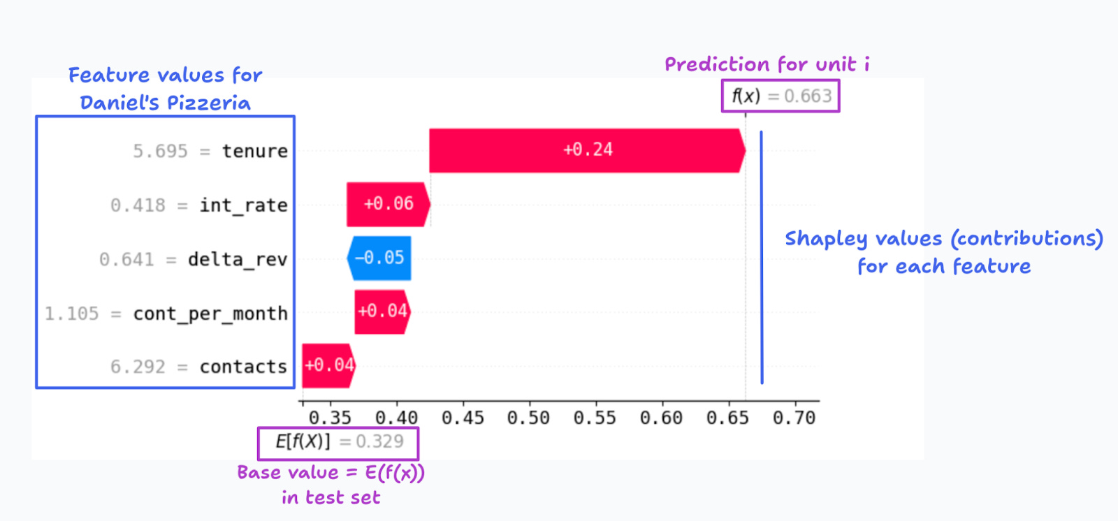
Since the data is simulated, we can compare the signs of the Shapley decomposition with those of the true DGP (Table 0). Compared to the average SMB in the sample, Daniel’s Pizzeria had lower tenure, so in the model, it should have a higher default probability, as the corresponding SHAP value

Final comments
Interpretability is an important skill that every data scientist should develop, as it plays an important role in model improvement, storytelling, fairness, and more. In this post I showed some popular methods to gain some insights into the workings of the model, and achieve a better understanding of the underlying true data generating process. In a later post I’ll describe mechanistic interpretability, that has become somewhat fashionable to open the black box of large language models.
I’m not endorsing this method. In chapter 15 of THP I endorse a model- or data generating process-based approach to feature engineering.
If you’re interested, check the Fairness and Machine Learning book, by Solon Barocas and coauthors.
Chapter 9 in THP provides a primer on simulation for ML
Caution! This is not as straightforward as it sounds! Observational data has many biases, and your model may inherit some or all of these, thus making you behave suboptimally. See the last chapter of Analytical Skills.
Don’t let this DAG fool you. While it is true operationally speaking – it correctly captures the true underlying DGP – in real life these features are proxies for the true underlying causes. See the notebook for some plausible stories about these underlying causes.
But you’re invited to check THP to learn about ALE
If interested, you can check Section 9.6 in Molnar’s book, or Chapter 8 in Biecek and Tomasz book. I’ve also found these lecture notes useful.