
Interpretable Machine Learning with Shapley Values


TL;DR
Shapley values are commonly used by data scientists to gain insights into the predictive behavior of their machine learning models. By design, Shapley values can provide both local and global interpretability. However, they are computationally expensive, as they require the computation of a sum that grows exponentially with the number of features in the model. In this post, I demonstrate how they work and calculate them for a sufficiently small simulated dataset. This ‘do-it-yourself’ approach can help you understand the intricacies of the method. I also show how you can test whether they yield intuitive results by using simple toy datasets.
Introduction
In a previous post, I used Shapley values as a technique to glean insights into local interpretability. This method has gained significant popularity among data scientists that want to report on local and global interpretability, but many times they don’t know how to interpret them.
In this post I’ll use a technique used frequently in Data Science: The Hard Parts (THP), where I first simulate a simple model, code the algorithm myself and use one of the available open source libraries to check that things match. Simple models , often referred to as “toy models”, are excellent for building an understanding of a problem or method. Additionally, coding the algorithm yourself is crucial for grasping the intricacies of how they work.
You can check all of my calculations using this Colab notebook.
What are Shapley values
If you remember from the previous post, Shapley values are taken from cooperative game theory, where a team of M players cooperates to obtain a payoff, and our task is to find some way to split the payoff. Shapley values are a solution to this problem, and, conveniently, also satisfy some desirable properties:
Null player (Dummy): players who don’t contribute get zero payoffs.
Efficiency: the sum of all payoffs should equal the payoff for the coalition.
Symmetry: players with equal contributions get equal payoffs.
Linearity: the payoff for a player in a weighted game, is the weighted sum of the corresponding payoffs.1
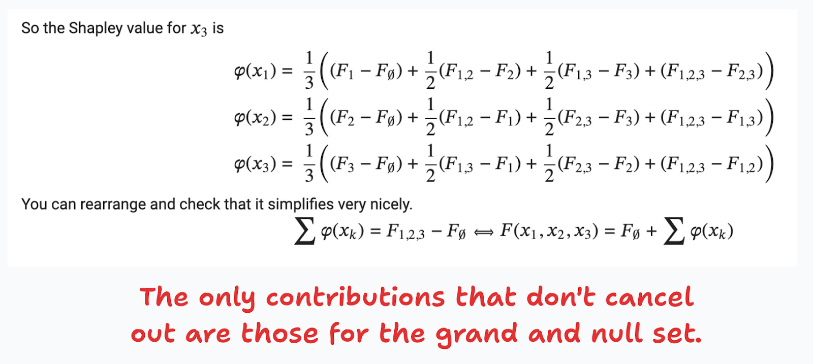
In machine learning (ML), features correspond to players, and the prediction plays the role of the payoff. We make predictions with a function F, and we want to find each feature’s contribution. Figure 0 shows that the Shapley value for a feature k, is the weighted average of the individual contributions across all possible subsets of features that exclude k.

Let’s compute the Shapley values for x3 in a model with only three features, x1, x2 and x3. Table 0 presents each of the necessary ingredients. The rows correspond to each of the subsets of the grand set, where x3 has been excluded: the null set, the singletons for x1 and x2, and the set that includes both of these features. The columns show the weights and the marginal contributions.
For instance, the null set has a weight of 1, given by the inverse of the binomial coefficient of 2 and 0, and the relative contribution is found by comparing the null prediction with the prediction when only the third feature is included. I’ll explain below what the “null prediction” is, but for now let’s assume that we can compute all of these predictions. If we add all of these terms, and divide by M we get the Shapley value.

Figure 1 shows you that if you add the Shapley values you recover the very important efficiency property that says that:
Individual prediction = Base value + SUM(feature contributions)
Computing Shapley values is computationally expensive
This is great, we are now ready to calculate Shapley values! Unfortunately this calculation grows exponentially with the number of features (Figure 2). For instance, if your model has 30 features, you will need to compute a sum over more than 1 billion terms! Since this is clearly infeasible, all modern methods attempt to reduce this complexity using different tricks.

But for the purposes of this post, in a simulated example with only three features, we can easily compute the Shapley values using the above formula.
Exact computation of Shapley values
When describing Table 0, I asked you to assume that we could make any prediction. Suppose you train a gradient boosting regression using our dataset that includes the three features. For any given combination of features (x1,x2,x3) you can then make a prediction with the corresponding predict() method. But you always need three values. How can we attempt a null prediction, or predictions on singleton sets, or any other subset of all features?
Figure 3 shows how this is done in practice. Whenever we need to make a prediction for a subset that doesn’t include the full set of features, we sample from the data to fill in the gaps. In this example, we need to make a prediction for the singleton set that includes only the third feature. We then sample with replacement from the data for each of the remaining features.

This approach works well, but since we’re using random sampling, we don’t want our Shapley values to depend on the result from one specific draw. To handle this we make many draws, and average out the predictions.
This explains why the base value is the same for all units, and why the SHAP library reports it as E(f(x)) (Figure 4). By making many draws, we can estimate the base value, and the Shapley decomposition is finally ready.

In Figure 5, I compare my calculations with the Shapley values obtained from the really great SHAP library. The closer a point is to the diagonal line, the better my calculation matches the library’s results. Naturally, since this is based on random draws, it’s highly unlikely that we’ll get the exact same result, but you see that both are in the same ballpark.

Can you change the base value?
As discussed, the base value is the prediction of the null coalition of having no features. We compute this by drawing (x1,x2,x3) triplets, making the corresponding predictions, and averaging out these predictions (E(f(x))).
But many times we would want to measure the contributions relative to some other baseline (B). Thanks to the linearity of the decomposition you can indeed make any given translation, and choose how to distribute the change across Shapley values. For instance, you can just translate them:
But notice that while the equality is kept, and you get something that looks like a Shapley decomposition, you lost the original interpretation of the decomposition. Indeed, some of the methods in the SHAP library allow you to change the base value, but my advice is to let go that temptation.2
From local to global interpretability
One great thing about Shapley values is that the decomposition applies for any given unit in the sample, so its computed at the unit level, thereby providing a tool for local interpretability.
For instance, for the unit in Figure 4, the Shapley decomposition shows that the third feature is the most important in explaining why the model predicts -19.7 instead of the base value of 0.4. This type of waterfall plot – or the alternative force plots – is quite common when presenting results for local interpretability using Shapley values.
Figure 6 shows another way to visualize global and local interpretability results. The left panel shows the average of the absolute values of the individual Shapley values, which can be used as a metric for global feature importance. The right panel displays a beeswarm plot, where individual Shapley values are plotted on the horizontal axis, and the color of the markers show the value of the feature for each unit. This additional dimension allows us to understand the directionality of the effects, as we did with Partial Dependence Plots3
For instance, units with large values for x1 and x3 also have large Shapley values, while the second feature displays a negative correlation. From here we can infer that x1 and x3 are positively correlated with the outcome, while x2 displays a negative correlation.

Testing our intuitions
Let’s check now if Shapley values generate results that are intuitive. To do so, I’ll simulate several linear models, train a gradient boosting regressor and plot some results. As stated in the introduction, I use this technique extensively in THP, since linear models have the advantage that they are both strongly locally and globally interpretable.
The first data generating process (DGP1) is:
DGP1 was designed such that we should not observe differences in feature importances, all of which are positively correlated with the outcome, with the exception of the second one. The first three panels of Figure 7 plot the Shapley values against the feature values, accompanied by the true unobserved slope parameter. The final plot reveals that all variables have similar feature importances. However, contrary to our expectations, the last feature displays a slightly larger importance.

I will finish with two additional simulations: in the first one, the slope parameter for x3 twice as large, and in the second one, I double the variance of the distribution from which the feature is drawn (x3 ~ N(0,2)). In the first case (DGP2), I expect the third feature to be twice as important as the other two variables. In the second case (DGP3), I expect the importance to increase less than proportionally (exactly by the square root of 2). Figure 8 shows that the results correspond to these intuitions.

Final comments
Shapley values are an excellent tool in the ML interpretability toolkit. They provide both local and global interpretability metrics, aiding in understanding the prediction behavior of your model. However, the method is computationally expensive, as it requires making predictions for all possible combinations of features, which grows exponentially with the number of features. Many implementations, not discussed here, aim to circumvent this problem, but it’s still advisable to use them with caution. For those interested in the computational aspect and exploring many of the capabilities of the SHAP library in Python, Lundberg et al. (2019) is a great reference.
This is somewhat cryptic, but loosely speaking this means that the value function is linear.
For instance, you can change the value in the shap.force_plot() and shap.decision_plot() allow you to do it. See this conversation where one of the authors of the paper and library explains how to also achieve this for visualization purposes.
With the SHAP library, you can use `shap.plots.bar()` and `shap.plots.beeswarm()` to get these plots.