


Machine Learning and Decision-Making: the case for Customer Acquisition Cost Optimization


TL;DR
The customer acquisition cost (CAC) is a key metric used by Marketing teams to quantify the effort in acquiring an average customer in a campaign.
In this post I discuss how you can use supervised machine learning to predict the CAC for your marketing campaign
Alternatively, for a given CAC target, you can reverse engineer the problem and find the number of leads you need to include in your campaign, along with the estimated total cost.
I also show how that the CAC is inversely related to the Precision of your classification model.
Introduction
In Chapter 14 of Data Science: The Hard Parts I discuss the case of simple and optimal thresholding, whereby one makes a binary decision depending on the value of the predicted outcome. In this post I want to expand on this idea, with the specific application to optimizing the customer acquisition cost.
What is the customer acquisition cost
The customer acquisition cost (CAC) is a metric commonly used by organizations to quantify the effort required to bring one additional customer to the company. It's calculated as the ratio of total spend to the number of new customers, interpreted as the average cost per customer for any acquisition campaign:
In a typical campaign, the marketing team first decides the budget (the numerator) and only then they choose the actual communication strategy, that may involve very complex decisions such as which channels to use, number of contact attempts per user, and potentially the whole communication journey.
Here I’ll start with the simplest framework where there’s only one contact per customer. It can be generalized to multiple contacts and channels, but following one of the mottos from Analytical Skills for AI and Data Science, I’ll be satisfied for now with this degree of simplification.
According to one study by Shopify, in 2024, CAC was as low as $21 per user in the Arts and Entertainment industry, and as high as $377 in the Electronics sector, and many such estimates can be found elsewhere on the web.
From an optimization point of view, once you set the budget, your task is to minimize the CAC by bringing in as many new customers as possible. Alternatively, you may wish to fix the CAC at some desired level, and target specific customers to achieve that level. I will pursue this latter path in what follows.
Classification and CAC
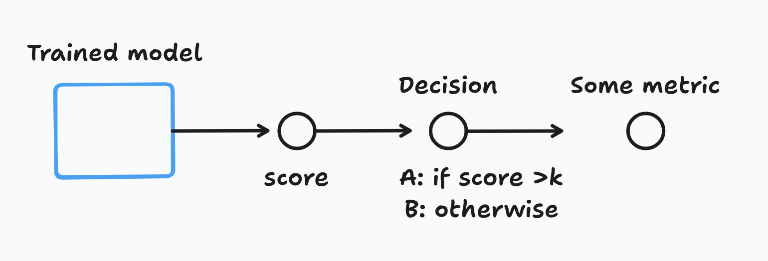
Consider a typical scoring conversion funnel, where the data scientist trains a classification model that predicts if a candidate will try the product or not. Since the whole idea of using a model is predictive targeting, they first score a pool of leads (L), and then send a subset to the Marketing team for communications to be delivered. Of these some will actually end up being converted into new customers.
The size of the subset is typically chosen using predictive performance and budgetary concerns. It’s not uncommon for the marketing team to fix the budget from the outset, which implicitly also fixes the number of candidates (PP ) from the pool to be contacted. The data scientist can then go and select PP leads that makes sense from a predictive performance point of view.
One way to do this is to think in terms of the precision of the model, that is, out of those PP candidates, how many are actually converted. When evaluating the performance of a classification model, I like to split the test sample into quantiles (say deciles), and plot the precision for each quantile. If the score is informative of the true conversion probability, this metric should grow across quantiles of score. Alternatively, one can think of sorting the units in the test sample using the score, and choosing the top k%. If the model is good, this top k% will have the largest possible precision, and the data scientist can then send this subset to the marketing team. This gives an expression for the denominator in the CAC definition.

Turning now to the numerator, one can easily reexpress it as the average unit cost (c) times the number PP of contacted users in the campaign, so we can finally express the CAC as a function of unit cost and the model’s precision:
There are several ways to use this expression.
Estimate your CAC ex-ante: given a budget and a model, you can estimate ex-ante your CAC just by plugging in the corresponding terms.
Estimate the size of your campaign: alternatively, you can solve for
k(implicitly defined by the precision of the model), and check if a target CAC can be achieved with your model, and how many customers will have to be touched. You can then answer questions like: “if Marketing has a dual target of acquiring Y customers each month, at a target CAC of X dollares, is this actually attainable with the current version of our models?”
While the the first use case is relatively straightforward there are indeed some subtleties that may arise. I will discuss below one such problem that you may encounter in practice.
The second use case tells you what’s achievable with your current iteration of the classification model. Suppose that Marketing tells you that they need to ensure a CAC of X dollars. Can you do it? Divide the unit cost by X and check if your model is able to deliver this precision. For instance, it could be that your sample size is so small, that the Marketing team may wish to reevaluate the budget for the campaign.
Calibrating your Precision estimates
Everything sounds easy enough: I have a classification model used to target specific customers, and I can then calibrate the CAC or the quantiles, depending on the budget and predictive performance of the model. What can go wrong?
Well, everything depends on whether you have a reliable estimate for the model’s precision. You can check this in at least the following two ways:
Calibrate the precision curve with an A/A test
Ensure that time windows are consistent
The first way is pretty straightforward: before predicting the CAC, test the model to get an empirical estimate of the precision curve. To do this, you can score your candidates pool, and sample from different quantiles for communication. You can then reconstruct the empirical precision curve.
However, you may be wondering if this is really necessary, given that, absent data and model drift, at training time you already have a test sample to get unbiased estimates for the model’s precision. I’ve found that this indeed works, but the data scientist needs to be super careful about using comparable time windows. I’ve use this windowing technique to control the simplest cases of data leakage1, but I also find it useful in the present context.
The idea is as follows: suppose that your campaign goes live tomorrow, so you decide to score the leads today. I call “today” the scoring time, and it splits the time period into two windows: looking forward, you have the prediction window, that defines the period you will use to evaluate your outcome (i.e. conversion or not). Looking backwards you have the observation window, where you measure some features that will allow you to predict your outcome into the future.
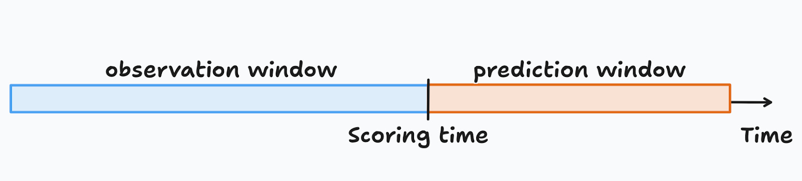
The observation window plays no relevant role in this discussion, so I will focus only on the prediction window. The main point I want to make is that the data scientist needs to ensure that the prediction window used at training time, matches the prediction window when the campaign is launched.
One thing that may happen is that the data scientist collects historical information for the outcome, say from the past six months, but the campaign is evaluated on a weekly basis. At the time of training the model you end up giving each unit up to six months to convert, but when the actual campaign is launched this period is restricted to a week. If you compare the precision estimates, you’ll find that the former is several times larger than the latter, which naturally underestimates your CAC.
What’s next
Since I used an average unit cost in the derivations, you can easily adapt this to cases where you may have a mix of channels and multi-touchpoint journeys. For instance, suppose that you use two different channels, the most expensive one once in the first eight hours, and the cheaper one twice in the next few days. As long as you have an estimate of the average unit cost, you’re then good to go and use the above derivation.
But now you may wish to also augment this analytical infrastructure to assess the optimality of one channel against some other alternatives. I’ll leave this topic for a future post.
An application of this windowing technique to data leakage can be found in Chapter 11 of Data Science; The Hard Parts.