
Machine Learning and Compression


A few months ago, a paper showed how a combination of gzip compression and nearest neighbors could outperform large language models (LLMs) in text classification tasks. Later, DeepMind researchers showed that LLMs can be used as lossless compressors for text, image and audio data.
In this post I want to discuss the connection between machine learning (ML) and compression. As David J.C. MacKay points in Information Theory, Inference, and Learning Algorithms, “data compression and data modeling are one and the same”, so it may not come as a surprise that ML and compression are indeed closely related.
Compression
Loosely speaking, the objective of a compressor is to reduce the size of a file or message, without losing “too much” information content. Lossless compressors achieve size reductions without any loss in information, and with lossy compressors there’s an actual trade-off between the two.1 The information content is measured using Shannon’s information entropy.
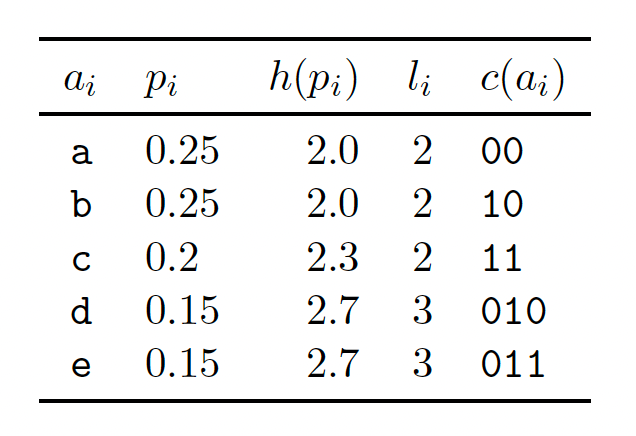
One example of a lossless compression algorithm is the Huffman coding algorithm. It proceeds by encoding each symbol separately, by first calculating the occurrence probability for each symbol and then assigning an encoding. The length of this encoding is inversely proportional to the symbol’s probability.
This can be seen in Figure 0, taken from Table 5.5 of McKay (2003), for the case of a five symbols alphabet {a,b,c,d,e}. Other than the first column, the remaining ones show (i) the probabilities of occurrence, (ii) Shannon’s information content, the optimal lengths2 and the actual encodings. Note that symbols with a lower probability of occurrence (d,e) have longer encodings. A string like aabae would then be encoded as the concatenation of the encoded symbols, in this case 00001000011.
A more powerful lossless compressor that achieves a near optimal length is arithmetic coding.3 Similar to the Huffman algorithm, it also needs an underlying probability model for the occurrence of symbols, so in a sense, both convert prediction into compression. The technical details are more complex, but at a very high-level this algorithm requires:
The probability of a symbol occurring, given the full history of preceding symbols.
A method that converts probabilities into subintervals in the unit interval.
I’ll illustrate how the algorithm works now. Say we want to encode abbabbb. A prerequisite is that we know all of the symbol wise unconditional and the one-step ahead conditional probabilities:
At the first step we want the unconditional probability of each symbol occuring. We can map these probabilities to subintervals that partition the unit interval, each with length equal to that probability. This same principle will apply at each subsequent step, but we will now be working on conditional probabilities. For instance, at the second step, since a has already occurred we partition the corresponding subinterval (from the previous step) into further subintervals, each with length proportional to the probabilities P(.|a). The algorithm continues in this fashion until you reach the end of the string, and the encoding is an interval contained in the final subinterval.
This algorithm is interesting, not only because of its near-optimality, but because it will play an important role in the DeepMind paper discussed later. The key insight to remember is that arithmetic coding uses a model for the conditional probabilities (Equation 1) that corresponds very closely to the probabilities used in autoregressive language models.
Compression for text classification
Imagine that instead of training large language models for a text classification task, you could just use a compressor, like gzip, and out-of-the-box nearest neighbors, without a substantial loss in predictive performance. This is exactly what Jiang, et.al propose in their paper, so you can imagine that it created quite a buzz in the AI community.4
Suppose you have training and test samples for a text classification task such as sentiment analysis. Importantly, your training sample is labeled, with each review associated with one sentiment (Figure 1). Our objective is to attach a sentiment to each review in the test sample. The idea pursued in the paper is to use a “similarity” criterion.
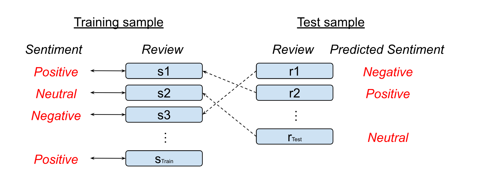
Suppose that we have such a way to assess the similarity of two reviews. For the first review in the test sample (r1), we go and look for the most similar review in the train sample (s3), and attach the corresponding sentiment as a prediction (negative). As you may notice, this is just k-nearest neighbors (k-NN) applied to a classification setting, with k=1. Of course, nothing constrains you from using some sort of majority voting for the case of k>1.
The authors use compression to construct a “similarity” metric. To see how this works, take two strings s1 and s2. Intuitively, if they are similar the size of the compressed version of their concatenation s1+s2 should be very close to the size of the compressed versions of s1 or s2.
Thus, they use the following Normalized Compression Distance as a similarity metric, where C(x) is the compressed length of x:
They derive this equation from information theoretic principles, but the intuition is the same as before: compression takes advantage of any redundancies in the symbols used.
The following Python snippet (closely based on the code provided in the paper) shows how the process works.5
def gzip_classifier(test_set, training_set):
  test_class = []
  for x1 in test_set:
    Cx1 = len(gzip.compress(x1[0].encode()))
    distance_from_x1 = []
    for x2 , _ in training_set:
      Cx2 = len(gzip.compress(x2[0].encode()))
      x1x2 = " ". join([ x1[0] , x2[0] ])
      Cx1x2 = len(gzip.compress(x1x2.encode()))
      ncd = (Cx1x2 - min( Cx1 , Cx2)) / max(Cx1 , Cx2 )
      distance_from_x1.append(ncd)
    sorted_idx = np.argsort(np.array(distance_from_x1))
    # use the top-1 class as the prediction
    top_1_class = training_set[sorted_idx[0]][1]
    test_class += [(x1,top_1_class)]
  return test_class

training_set = [("I'm very happy with this entry",'positive'), ("The food at the restaurant was terrible","negative")]
test_set = [("I'm happy with the movie",''),("I really disliked their 'happy' menu.  It's better suited for kids.", "")]

classifier = gzip_classifier(test_set, training_set)
for k in classifier:
  rev_k = k[0][0]
  class_k = k[1]
  print(f'Review: {rev_k} --> sentiment = {class_k}')

''' prints:
Review: I'm happy with the movie --> sentiment = positive
Review: I really disliked their 'happy' menu.  It's better suited for kids. --> sentiment = positive
'''
This example highlights one of the main problems with the suggested algorithm (and the authors acknowledge this). Consider the two reviews:
s1 = ‘I'm very happy with this entry‘
s2 = ‘I really disliked their “happy” meal‘
I suspect that any human would classify them as positive and negative, just as GPT-4 did when I prompted it. But since the compression-based similarity metric works on text redundancies and not on semantic similarity, you end up with the latter being classified as positive.6
To sum up, the good news is that compression can take you a long way if you want to do text classification. The bad news is that k-NN is computationally expensive for large datasets, and that you may get bad performance since it’s not based on semantic similarity.
LLMs as lossless compressors
If the previous paper argued that compressors can act as language models for specific tasks, in Language Modeling as Compression, DeepMind researchers Delétang, et.al. make the converse assertion that LLMs can be used as lossless compressors. The key insight is that by minimizing the log-loss, current autoregressive language models also achieve maximal compression. As the authors state:
(C)urrent language model training protocols use a maximum-compression objective.
The authors use arithmetic coding as their compressor algorithm to move from prediction to compression. As described in the first section, to encode a sentence like “I want to encode this sentence” we require the probabilities for the next word or token conditioning on the history or context, and an algorithm that maps these probabilities to intervals. The latter is given by arithmetic coding, and the former is the result of training language models. It’s in this sense that the authors are able to convert an LLM into a compressor. They train several relatively small LLMs and also use several of the larger Chinchilla models (see this post). They then compare the results with standard general compressors like gzip and LZMA2, as well as more specialized ones for images and audio data, such as PNG and FLAC.
The main result is that all of the transformer-based models perform as well, or even better than, the alternatives, with the larger Chinchilla 70B model emerging as the overall winner. This is true for their raw compression rate (compressed size / raw size), but the advantange of large model disappears once they adjust for the size of the model. In practice, this means that using LLMs for compression is an overkill: you get superior compression performance at the expense of usability. Please note that the paper has many other interesting results. In this discussion, however, I wanted to specifically highlight the role that language modeling might play in compression.
Machine learning and compression
Up to now I’ve discussed a direct connection between compression and ML, but ML is itself a form of lossy compression: we create models that learn about a complex world using any underlying patterns and redundancies in the data with the objective to minimize the predictive error.
Suppose I want to compress the numbers:
141.0, 76.7, 35.7, 12.9, 2.8, 0.4, 0.3, -2.8, -14.2, -39.0The ML approach would be to fit a model on the data to minimize the loss. With a parametric model, compression is then given by providing a mapping from inputs and parameters to data.
Suppose I give you {inputs, parameters} instead of the data. Have I achieved any compression, even if lossy? What about if I only give you {parameters}?
From a data compression perspective, it’s unlikely that the answer to the first question is positive.7 On the other hand, if we could just use the parameters to make a sufficiently good prediction, we would most certainly achieved some sort of compression (assuming that the if the model isn’t overly overparametrized). Interestingly, this is what happens when we prompt an autoregressive LLM.
Is it possible to compress all the knowledge on the web? In a somewhat loose sense that’s what LLMs like GPT-4 have already achieved. Recall that by applying a sufficient degree of overparameterization, these models can almost completely memorize the training set. Along the way, they also achieve remarkable feats in reasoning, language understanding, and generation. It’s no surprise, then, that GPT-4 and other LLMs achieve impressive results in a diverse set of standardized tests.
To sum up, ML is in itself a form of lossy compression, so it won’t be surprising if researchers keep coming up with novel ways to highlight their relationship.
To make things less abstract, think of what happens when you compress a file and send it by email. In this case, you expect two things to happen: (i) the size of the compressed file is smaller, and (ii) the decompressed file is an exact copy of the original so there was no loss.
Shannon’s information content is defined as -log(1/p), with the log in base 2. The optimal length is given by the ceiling of the information content.
Shannon’s source coding theorem establishes that information entropy is the absolute best that can be achieved in terms of compression. Arithmetic coding is always at most two bits away from that optimum. See McKay, p.115.
To be fair, the use of compressors for classification had been known since at least 2000. See the Related Work section in the DeepMind paper. Jiang, et.al. also provide some historical context when discussing their relative contribution.
Since this is k-NN, you can immediately check that the algorithm is computationally expensive: it requires O(nm) operations, where n,m are the sizes of the training and test samples), so for large datasets it may not be advisable to use.
Of course, with a larger dataset and optimizing the hyperparameter that controls the number of neighbors, you can trade-off some of the bias for some variance and try to come up with a practical workaround for this problem.
But this might be achieved by reducing the precision of inputs and parameters and accept the lower performance as part of the loss of the compressor.